A small Tutorial
(Draft)
Sven Eric Panitz
TFH Berlin
Version Sep 24, 2004
Publish early and publish often. That is the reason why you can read this. I started playing around with HOpenGL the Haskell port of OpenGL a common library for doing 3D graphics. I more or less took minutes of my efforts and make them public in this tutorial. I did not have any prior experience in graphics programming, when I started to work with HOpenGL.
The source of this paper is an XML-file. The sources are processed by
an XQuery processor, XSLT scripts and LATEX
in order to
produce the different formats of the tutorial.
I'd like to thank Sven Panne1, the author of HOpenGL,
who has been so kind to
comment on first drafts of this tutorial.
Contents
1 Introduction1.1 A Little Bit of Practice
1.1.1 Opening Windows
1.1.2 Drawing into Windows
1.2 A Little Bit of Theory
1.2.1 Haskell
1.2.2 OpenGL
1.2.3 Haskell and OpenGL
1.3 A Little Bit of Technics
1.4 A Little Bit of History
2 Basics
2.1 Setting and Getting of Variables
2.1.1 Setting values
2.1.2 Getting values
2.1.3 Getting and Setting Values
2.1.4 What do the variables refer to
2.2 Basic Drawing
2.2.1 Display Functions
2.2.2 Primitive Shapes
2.2.3 Curves, Circles and so on
2.2.4 Attributes of primitives
2.2.5 Tessellation
2.2.6 Cubes, Dodecahedrons and Teapots
3 Modelling Transformations
3.1 Translate
3.2 Rotate
3.3 Scaling
3.4 Composition of Transformations
3.5 Defining your own transformation
3.5.1 Shear
3.6 Some Word of Warning
3.7 Local transformations
4 Projection
4.1 The Function Reshape
4.2 Viewport: The Visible Part of Screen
4.3 Orthographic Projection
5 Changing States
5.1 Modelling your own State
5.2 Handling of Events
5.2.1 Keyboard events
5.3 Changing State over Time
5.3.1 Double buffering
5.4 Pong: A first Game
6 Third Dimension
6.1 Hidden Shapes
6.2 Perspective Projection
6.3 Setting up the Point of View
6.3.1 Oribiting around the origin
6.4 3D Game: Rubik's Cube
6.4.1 Cube Logics
6.4.2 Rendering the Cube
6.4.3 Rubik's Cube
6.5 Light
6.5.1 Defining a light source
6.5.2 Tux the Penguin
Chapter 1
Introduction
In this chapter some basic background information can be found. You you
can read the sections of this chapter in an arbitrary order. Whatever
your personal preference is.
1.1 A Little Bit of Practice
Before you read a lot of technical details you will probably like to
see something on your screen. Therefore you find some very simple
examples in the beginning. This will give you a first impression, of how
an OpenGL program might look like in Haskell.
1.1.1 Opening Windows
OpenGL's main purpose is to render some graphics on a device. This
device is generally a window on your computer screen. Before you can
draw something on a screen you will need to open a window. So let's
have a look at the simpliest OpenGL program, which just opens an empty
window:
HelloWindow
import Graphics.UI.GLUT
import Graphics.Rendering.OpenGL

main = do
  getArgsAndInitialize
  createAWindow "Hello Window"
  mainLoop

createAWindow windowName = do
  createWindow windowName
  displayCallback $= clear [ColorBuffer]
The first two lines import the necessary libraries. The main function
does three things:
- initialize the OpenGL system
- define a window
- start the main procedure for dispaying everything and reacting on events
For the definition of a window with a given name we do two things:
- create some window with the given name
- define, what is to be done, when the window contents is to be displayed. In the simple example above we simply clear the screen of any color by filling it with the default background color.
This 10 lines can be compiled with ghc. Do not forget to
specify the packages, which contain the OpenGL library. It suffices to
include the package GLUT, which automatically forces the
inclusion of the package OpenGL. GLUT is the graphical user
interface, which comes along with OpenGL, i.e. the window managing
system etc.
sep@swe10:~/hopengl/examples> ghc -package GLUT -o HelloWindow HelloWindow.hs
sep@swe10:~/hopengl/examples> ./HelloWindow
When you start the program, a window will be opened on your desktop. As you
may have noticed, we did not specify any attribute of the window, like
its size and position. GLUT is defined in a way that initial default
values are used for unspecified attributes.
1.1.2 Drawing into Windows
The simple program above did just open a window. The main purpose of
OpenGL is to define some graphics which is rendered in a window.
Before starting to systematically explore the OpenGL library let's
have a look at two examples that draw something into a window frame.
Some Points
First we will draw some tiny points on the screen.
We use the same code for openening some window:
SomePoints
import Graphics.UI.GLUT
import Graphics.Rendering.OpenGL

main = do
  (progName,_) <- getArgsAndInitialize
  createAWindow progName
  mainLoop
The only thing that has changed, is that we make use of one of the values returned by getArgsAndInitialize: the name of the program.
For the window definition we use the code from HelloWindow.hs. But instead of clearing the screen, when the
window is to be displayed, we use an own display function:
SomePoints
createAWindow windowName = do
  createWindow windowName
  displayCallback $= displayPoints
We want to draw some points on the screen. So let's define some
points. We can do this in a list. Points in a three dimensional space
are triples of coordinates. We can use floating point numbers for
coordinates in OpenGL.
SomePoints
myPoints :: [(GLfloat,GLfloat,GLfloat)]
myPoints =
  [(-0.25, 0.25, 0.0)
  ,(0.75, 0.35, 0.0)
  ,(0.75, -0.15, 0.0)
  ,((-0.75), -0.25, 0.0)]
Eventually we need the display function, which displays these points.
SomePoints
displayPoints = do
  clear [ColorBuffer]
  renderPrimitive Points
    $mapM_ (\(x, y, z)->vertex$Vertex3 x y z) myPoints
As you see, when the window ist displayed, we want first everything to
be cleared from the window. Then we use the HOpenGL function renderPrimitive. The first argument Point specifies
what it is that we want to render; points in our case. For the second
argument we need to transform our coordinates into some data, which is
used by HOpenGL. Do not yet worry about this transformation.
As before, you will notice that again for quite a number of
attributes we did not supply explicit values. We did not specify the
Color of the points to be drawn. Moreover we did not define the
coordinates of the graphics window. Looking at its result it is
obviously a two dimensional
view, where the lower left corner seems to have coordinates (-1,-1) and the
upper right corner the (1,1). These values are default values chosen
by the OpenGL library.
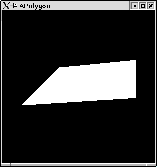
A Polygon
The points in the last section were rather boring? By changing a
single word, we can span an area with these points. Instead of saying
render the following as points, we can tell HOpenGL to render them as
a polygon.
Example:
So here the program from above with one word changed. Points becomes Polygon.
APolygon
import Graphics.UI.GLUT
import Graphics.Rendering.OpenGL

main = do
   (progName,_) <-getArgsAndInitialize
   createAWindow progName
   mainLoop

createAWindow windowName = do
   createWindow windowName
   displayCallback $= displayPoints

displayPoints = do
  clear [ColorBuffer]
  renderPrimitive Polygon
    $mapM_ (\(x, y, z)->vertex$Vertex3 x y z) myPoints

myPoints :: [(GLfloat,GLfloat,GLfloat)]
myPoints =
  [(-0.25, 0.25, 0.0)
  ,(0.75, 0.35, 0.0)
  ,(0.75, -0.15, 0.0)
  ,((-0.75), -0.25, 0.0)]
The resulting window can be found in figure 1.1.
1.2 A Little Bit of Theory
1.2.1 Haskell
Haskell [] is a lazily
evaluated functional programming language. This
means that there are no mutable variables. A Haskell program consists
of expressions, which do not have any side effects. Expressions are
only evalutated to some value when this is absolutely necessary for
program execution. This means it is hard to predict in which order
subexpressions get evaluated.
Expressions
evaluate to some value without changing any state. This is a nice
property of Haskell, because it makes reasoning about programs easier
and programs are very robust.
1.2.2 OpenGL
OpenGL on the other hand is a graphics library which is defined in
terms of a state machine. A mutable state modells the current
state of the world. Functions are executed one after another
on this state in
order to modify certain variables. E.g. one variable keeps the current
color to which all drawing statements refer. There is a statement
which allows to set the color variable to some other value.
A comprehensive introduction to OpenGL can be found in the so calledredbook[]. OpenGL comes along with
a utility library called GLU [] and a system
independent GUI library called GLUT [].
1.2.3 Haskell and OpenGL
Having said this, Haskell and OpenGL seem to cooperate badly. There
seems to be a great mismatch between the fundamental concepts of the two.
However,
the designers of Haskell discovered a very powerful structure, which is
a perfect concept for modelling state changing functions in a purely
functional language: Monads[]. Most
Haskell programmers do not
worry about the theory of monads but simply use them, whenever they
do I/O, state changing functions or in parser construction. With
monads functional programs can almost look like ordinary imperative
progams [].
Monads are so essential to functional programming, that they have a
special syntactic construct in Haskell, the do notation.
Consider the following simple Haskell program, which uses monads:
Print
main = do
  let x = 5
  print x
  let x = 6
  print x
  xs  <- getLine
  print (length xs)
The monadic statements start with the keyword do. The statements have side effects. Variables can be defined and redefined in let-expressions2. Monadic statements can have a result. This can be retrieved from the statement by the <- notation.
On another aspect OpenGL and Haskell perfectly match. In OpenGL
functions are assigned to different data objects,
e.g. a display function is passed to windows. Since
functions are first class citizens, they can easily and type safe be
passed around3.
1.3 A Little Bit of Technics
If you want to start programming OpenGL in Haskell you need to be one
of the brave, who compile sources from the functional programming CVS
repository in Glasgow. There is not yet a precompiled version of the
current HOpenGL library. Go to
the website (www.haskell.org/ghc) of the Glasgow
Haskell Compiler (GHC), follow closely the instructions on the
page CVS cheat sheet. When doing the ./configure step, then use the option --enable-hopengl. i.e. start the
command ./configure --enable-hopengl. This will ensure
that the Haskell OpenGL library will be build and the packages OpenGL and GLUT are added to your GHC installation.
To compile Haskell OpenGL programs you simply have to add the
package information to he command line invocation of GHC,
i.e. use:
ghc -package GLUT MyProgram.hs
ghc -package GLUT MyProgram.hs
Everything else, linking etc is done by GHC. You do not have to worry
about library paths or anything else.
1.4 A Little Bit of History
The Haskell port of OpenGL has been done by Sven Panne. Currently a
stable version exists and can be downloaded as precompiled
binary. This tutorial deals with the completely revised version of
HopenGL, which has a more Haskell like API and needs less technical
overhead. This new version is not yet available as ready to use
package. You need to compile it yourself.
This tutorial has been written with no prior knowledge of OpenGL and
no documentation of HOpenGL at hand.
For the old version 1.04 of HOpenGL an online tutorial written
by Andre W B Furtado exists
at (www.cin.ufpe.br/~haskell/hopengl/index.html) .
Chapter 2
Chapter 2
Basics
2.1 Setting and Getting of Variables
From what we have learnt in the introduction, we know that we are
dealing with a state machine and will write a sequence of monadic
functions which effect this machine. Before we start drawing fancy
pictures let us explore the way values are set and retrieved in
HOpenGL.
2.1.1 Setting values
The most basic operation is to
assign values to variables in the state machine. In HOpenGL this is
done by means of the operator $=4 You do not need to understand, how this
operator is implemented. You simply can imagine that it is an
assignment operator. The left operand is a variable which gets
assigned the right operand. We can revisit the first program, which
simply opened a window.
Example:
When we have created a window, we assign a size to it:
Set
import Graphics.UI.GLUT
import Graphics.Rendering.OpenGL

main = do
  getArgsAndInitialize
  myWindow "Hello Window"
  mainLoop

myWindow name = do
  createWindow name
  windowSize $= Size 800 500
  displayCallback $= clear [ColorBuffer]
One example of the assignment operator we have allready seen. In the
last line we assign a function to the variable displayCallback. This function will be executed, whenever the
window is displayed.
As you see, more you do not need to know about $=. But if you
want to learn more about it read the next section.
Implementation of set
The operator $= is defined in the module
Graphics.Rendering.OpenGL.GL.StateVar as a member function of a type class:
Graphics.Rendering.OpenGL.GL.StateVar as a member function of a type class:
infixr 2 $=

class HasSetter s where
   ($=) :: s a -> a -> IO ()
The variables of HOpenGL, which can be set are of
type SettableStateVar e.g.:
windowTitle :: SettableStateVar String. Further variables that can be set for windows are: windowStatus, windowTitle, iconTitle, pointerPosition,
windowTitle :: SettableStateVar String. Further variables that can be set for windows are: windowStatus, windowTitle, iconTitle, pointerPosition,
2.1.2 Getting values
You might want to retrieve certain values from the state.
This can be done with the function get, which is in
a way the corresponding function to the operator $=.
Example:
You can retrieve the size of the screen:
Get
import Graphics.UI.GLUT
import Graphics.Rendering.OpenGL

main = do
  getArgsAndInitialize
  x<-get screenSize
  print x
When you compile and run this example the size of your screen it printed:
sep@swe10:~/hopengl/examples> ghc -package GLUT -o Get Get.hs
sep@swe10:~/hopengl/examples> ./Get
Size 1024 768
sep@swe10:~/hopengl/examples>
Implementation of get
There is a corresponding type class, which denotes that values can be
retrieved from a variable:
class HasGetter g where
   get :: g a -> IO a
Variables which implement this class are of type GettableStateVar a.
2.1.3 Getting and Setting Values
For most variables you would want to do both: setting them and
retrieving their values. These variables implement both type classes
and are usually of type: StateVar.
But things do not always work so simple as this sounds.
Example:
The following program sets the size of a window. Afterwards the variable windowSize is retrieved:
SetGet
import Graphics.UI.GLUT
import Graphics.Rendering.OpenGL

main = do
  getArgsAndInitialize
  myWindow "Hello Window"
  mainLoop

myWindow name = do
  createWindow name
  windowSize $= Size 800 500
  x<-get windowSize
  print x
  displayCallback $= clear [ColorBuffer]
Running this program gives the somehow surprising result:
sep@swe10:~/hopengl/examples> ./SetGet
Size 300 300
The window we created, has the expected size of (800,500) but the
variable windowSize still has the default value (300,300).
The reason for this is, that setting the window size state variable
has not a direct effect. It just states a wish for a window size. Only
in the execution of the function mainLoop actual windows will
be created by the window system. Only then the window size will be
taken into account. Up to that moment the window size variable still
has the default value. If you print the window size state within some
function which is executed in the main loop, then you will get the
actual size. By the way: you can try initialWindowSize without
getting such complecated surprising results.
2.1.4 What do the variables refer to
The state machine contains variables and stacks of objects, which are
effectedly mutated by calls to monadic functions. However not only the
get and set statements modify the state but also statements
like createWindow. This makes it in the beginning a bit hard
to understand, when the state is changed in which way.
The createWindow statement not only constructs a window
object, but keeps this new window as the current window in the
state. After the createWindow statement all window effecting
statements like setting the window size, are applied to this new
window object.
2.2 Basic Drawing
2.2.1 Display Functions
There is a window specific variable which stores the function
that is to be executed
whenever a window is to be displayed, the variable displayCallback. Since Haskell is a higher order language, it is
very natural to pass a function to the assignment operator.
We can define a function with some arbitrary name. The function can be
assigned to the variable displayCallback. In this function we
can define a sequence of monadic statements.
Clearing the Screen
A first step we would like to do whenever the window needs to be drawn
is to clear from it whatever it contains5. HOpenGL provides the
function clear, which does exactly this job. It has one
argument. It is a list of objects to be cleared. Generally you will
clear the so called color buffer, which contains the color displayed
for every pixel on the screen.
Example:
The following simple program opens a window and clears its content pane whenever it is displayed:
Clear
import Graphics.UI.GLUT
import Graphics.Rendering.OpenGL

main = do
  (progName,_) <- getArgsAndInitialize
  createAWindow progName
  mainLoop

createAWindow windowName = do
  createWindow windowName
  displayCallback $= display

display = clear [ColorBuffer]
First Color Operations
The window in the last section has a black background. This is because
we did not specify the color of the background and HOpenGL's default value
for the background color is black. There is simply a variable for the
background color.
For colors several data types are defined. An easy to use one is:
data Color4 a = Color4 a a a a
   deriving ( Eq, Ord, Show )
The four parameters of this constructor specify the red, green and blue values of the color and additionally a fourth argument, which denotes the opaqueness of the color. The values are usually specified by floating numbers of type GLfloat. Values for number attributes are between 0 and 1.
You may wonder, why there is a special type GLfloat for
numbers in HOpenGL. The reason is that OpenGL is defined in a way that
it is as independent from concrete types in any implementation as
possible.
However you do not have to worry too much
about this type. You can use ordinary float literals for numbers of
type GLfloat. Haskells overloading mechanism ensures that
these literals can create GLfloat numbers.
Example:
This program opens a window with a red background.
BackgroundColor
import Graphics.UI.GLUT
import Graphics.Rendering.OpenGL

main = do
  getArgsAndInitialize
  createAWindow "red"
  mainLoop

createAWindow windowName = do
  createWindow windowName
  displayCallback $= display

display = do
  clearColor $= Color4 1 0 0 1
  clear [ColorBuffer]
Committing Complete Drawing
Whenever in a display function a sequence of monadic statements is
defined, a final call to the function flush should be
made. Only such a call will ensure that the statements are completely
committed to the device, on which is drawn.
2.2.2 Primitive Shapes
So most preperatory things we know by now. We can start drawing onto the
screen. Astonishingly in OpenGL there is only very limited number of shapes
for drawing. Just points, simple lines and polygons. No curves or more
complicated objects. Everything needs to be performed with these
primitive drawing functions. The main function used for drawing
something is renderPrimitive. The first argument of this
functions specifies what kind of primitive is to be drawn. There are
the following primitives defined in OpenGL:
data PrimitiveMode =
     Points
   | Lines
   | LineLoop
   | LineStrip
   | Triangles
   | TriangleStrip
   | TriangleFan
   | Quads
   | QuadStrip
   | Polygon
   deriving ( Eq, Ord, Show )
The second
argument defines the points which specify the primitives. These points
are so called vertexes. Vertexes are actually monadic functions which
constitute a point. If you want to define a point in a 3-dimensional
universe with the coordinates x, y, z then you can use
the following expression in HOpenGL:
vertex (Vertex3 x y z)or, if you prefer the use of the standard prelude operator $:
vertex$Vertex3 x y z
Points
We have seen in the introductory example that we can draw
points. We can simply define a vertex and use this in the
function renderPrimitiv.
Example:
This program draws one single yellow point on a black screen.
SinglePoints
renderPrimitive Points$vertex$Vertex3 (0.1::GLfloat) 0.5 0
import Graphics.UI.GLUT
import Graphics.Rendering.OpenGL

main = do
  getArgsAndInitialize
  createAWindow "points"
  mainLoop

createAWindow windowName = do
  createWindow windowName
  displayCallback $= display

display = do
  clear [ColorBuffer]
  currentColor $= Color4 1 1 0 1
  renderPrimitive Points
     (vertex (Vertex3 (0.1::GLfloat) 0.5 0))
  flush
If you do not like parantheses then you can of course use the
operator $ from the prelude and rewrite the line:renderPrimitive Points$vertex$Vertex3 (0.1::GLfloat) 0.5 0
Unfortunately Haskell needs sometimes a little bit of help for
overloaded type classes. Therefore you find the type
annotation (0.1::GLfloat) on one of the float literals. In
larger applications Haskell can usually infer this information from
the context. Just in smaller applications you will sometimes need to
help Haskell's type checker a bit.
The second argument of renderPrimitive is a sequence of
monadic statements. So, if you want more than one point to be drawn,
you can define these in a nested do statement
Example:
In this program we use a nested do statement to define more points.
MorePoints
import Graphics.UI.GLUT
import Graphics.Rendering.OpenGL

main = do
  getArgsAndInitialize
  createAWindow "more points"
  mainLoop

createAWindow windowName = do
  createWindow windowName
  displayCallback $= display

display = do
  clear [ColorBuffer]
  currentColor $= Color4 1 1 0 1
  renderPrimitive Points $
   do

      vertex (Vertex3 (0.1::GLfloat) 0.6 0)

      vertex (Vertex3 (0.1::GLfloat) 0.1 0)
  flush
If you want to think of points mainly as triples then you can convert
a list of points into a sequence of monadic statements by first maping
every triple into a vertex, e.g. by:
map (\(x,y,z)->vertex$Vertex3 x y z)
and then combining the sequence of monadic statements into one monadic statement. Therefore you can use the standard function for monads: sequence_. The standard function mapM_ is simply the composition of map and sequence_, such that a list of triples can be converted to a monadic vertex statement by:
mapM_ (\(x,y,z) -> vertex$Vertex3 x y z)
which is the technique used in the introductory example.
Example:
Thus we can rewrite a points example in the following way: points are defined as a list of triples. Furthermore we define some useful auxilliary functions:
EvenMorePoints
import Graphics.UI.GLUT
import Graphics.Rendering.OpenGL

main = do
  getArgsAndInitialize
  createAWindow "more points"
  mainLoop

createAWindow windowName = do
  createWindow windowName
  displayCallback $= display

display = do
  clear [ColorBuffer]
  currentColor $= Color4 1 1 0 1
  let points = [(0.1,0.6,0::GLfloat)
               ,(0.2,0.8,0)
               ,(0.3,0.1,0)
               ,(0,0,0)
               ,(0.4,-0.8,0)
               ,(-0.2,-0.8,0)
               ]
  renderPoints points
  flush

makeVertexes = mapM_ (\(x,y,z)->vertex$Vertex3 x y z)

renderPoints = renderAs Points

renderAs figure ps = renderPrimitive figure$makeVertexes ps
Some useful functions
In the following we want to explore all the other different shapes
which can be rendered by OpenGL. All shapes are defined in terms of
vertexes which you can think of as points. We have allready seen how
to define vertexes and how to open a window and such things. We
provide a simple module, which will be used in the consecutive
examples. Some useful functions are defined in this module.
PointsForRendering
module PointsForRendering where
import Graphics.UI.GLUT
import Graphics.Rendering.OpenGL
A first function will open a window und use a given display function for the window graphics:
PointsForRendering
renderInWindow displayFunction = do
  (progName,_) <-  getArgsAndInitialize
  createWindow progName
  displayCallback $= displayFunction
  mainLoop
The next function creates for a list of points, which are expressed as
triples, and a basic shape a display function which renders the
desired shape.
PointsForRendering
displayPoints points primitiveShape = do
  renderAs primitiveShape points
  flush

renderAs figure ps = renderPrimitive figure$makeVertexes ps

makeVertexes = mapM_ (\(x,y,z)->vertex$Vertex3 x y z)
Eventually we define a list of points as example and provide a function for easy use of these points:
PointsForRendering
mainFor primitiveShape
 = renderInWindow (displayMyPoints primitiveShape)

displayMyPoints primitiveShape = do
  clear [ColorBuffer]
  currentColor $= Color4 1 1 0 1
  displayPoints myPoints primitiveShape

myPoints
 = [(0.2,-0.4,0::GLfloat)
   ,(0.46,-0.26,0)
   ,(0.6,0,0)
   ,(0.6,0.2,0)
   ,(0.46,0.46,0)
   ,(0.2,0.6,0)
   ,(0.0,0.6,0)
   ,(-0.26,0.46,0)
   ,(-0.4,0.2,0)
   ,(-0.4,0,0)
   ,(-0.26,-0.26,0)
   ,(0,-0.4,0)
   ]
Example:
We can now render the example points in a oneliner:
RenderPoints
import PointsForRendering
import Graphics.Rendering.OpenGL

main = mainFor Points
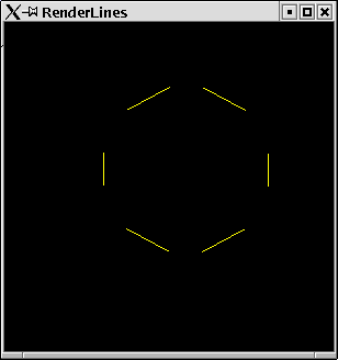
Lines
The next basic thing to do with vertexes is to connect them, i.e.
consider them as starting and end point of a line. There are three
ways to connect points with lines in OpenGL.
Singleton Lines
The most natural way is to take pairs of points and draw lines between these.
This is done in the primitive mode Lines. In order that this
works properly an even number of vertexes needs to be supplied to the
function renderPrimitive.
Line Loops
Example:
Connecting our example points by lines. Pairs of points define singleton lines.
RenderLines
import PointsForRendering
import Graphics.Rendering.OpenGL

main = mainFor Lines
The resulting window can be found in figure 2.1.
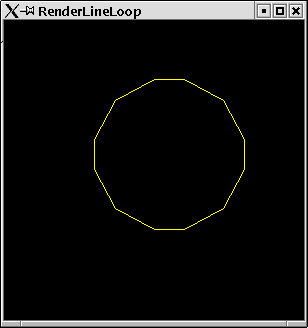
The next way to connect points with lines you probably can imagine is
to make a closed figure. The end point of a line is the starting point
of the next line and the last point is connected with the first, such
that a closed loop of lines is created.
Line Strip
Example:
Now we make a loop of lines with our example points.
RenderLineLoop
import PointsForRendering
import Graphics.Rendering.OpenGL

main = mainFor LineLoop
The resulting window can be found in figure 2.2.
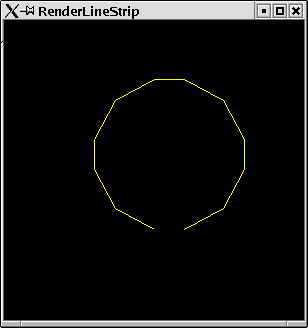
A strip of lines is very close to a loop of lines. The only thing
missing is the last line which connects the last point with the first
one again.
Example:
Now we make a strip of lines with our example points.
RenderLineStrip
import PointsForRendering
import Graphics.Rendering.OpenGL

main = mainFor LineStrip
The resulting window can be found in figure 2.3.
Triangles
The next basic shape which can be rendered by OpenGL are
triangles. Triples of points are taken and triangles are drawn with
these. As for lines there are three flavours of triangles.
Triangle
The most natural way of drawing triangles is to take triples and draw
triangles. In order to work for triangles, the number of points
provided needs to be a multiple of 3.
Triangle Strips
Example:
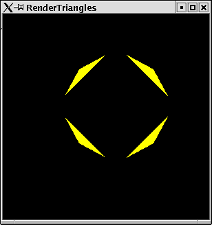
Our example vertexes define 12 points such that we get 4 triangles
RenderTriangles
import PointsForRendering
import Graphics.Rendering.OpenGL

main = mainFor Triangles
The resulting window can be found in figure 2.4.
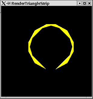
A triangle strip makes a sequence of triangles where the next triangle
uses two points of its predecessor and one new point.
TriangleFan
Example:
For our 12 points a triangle strip will create 10 triangles.
RenderTriangleStrip
import PointsForRendering
import Graphics.Rendering.OpenGL

main = mainFor TriangleStrip
The resulting window can be found in figure 2.5.
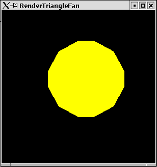
A fan has one starting point for all triangles. Triangles are always
drawn starting from the first point.
Example:
Our example points as a fan. 10 triangles are rendered.
RenderTriangleFan
import PointsForRendering
import Graphics.Rendering.OpenGL

main = mainFor TriangleFan
The resulting window can be found in figure 2.6.
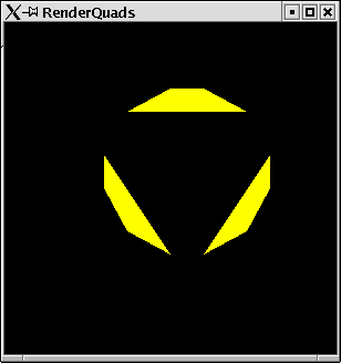
Quads
Lines connected two points, triangles three points, now we will connect
four points. This is calles a quad. There are two flavours of
quads.
Singleton Quads
The primitive mode Quads takes quadruples of points and
connects them in order to render a filled figure.
In a three dimensional world quads are unlike triangles not
necessarily plane areas.
Example:
For our 12 example points OpenGL renders 3 quads
RenderQuads
import PointsForRendering
import Graphics.Rendering.OpenGL

main = mainFor Quads
The resulting window can be found in figure 2.7.
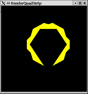
QuadStrips
For a strip of quads OpenGL uses two points of the preceeding quads
for the next quad. The number n of vertexes therefore
needs to be of the form: n=4+2*m.
Example:
Our examples vertexes now used for a strip of quads.
RenderQuadStrip
import PointsForRendering
import Graphics.Rendering.OpenGL

main = mainFor QuadStrip
Polygons
We connected two, three and for points. Eventually there is a shape
that connects an arbitrary number of points. This is generally called
a polygon. There are some restrictions for polygons:
- no convex corners are allowed.
- lines may not cross each other.
- polygons need to be planar.
Example:
Eventually our vertexes are used to define a polygon.
RenderPolygon
import PointsForRendering
import Graphics.Rendering.OpenGL

main = mainFor Polygon
In this case the resulting window looks like the triangle fan we have seen before.
If you want to render polygons which hurt some of the restrictions
above, you need to represent them by a set of smaller polygons. Since
this is a tedious task to be done manually there is a library
available, which does this for you: the GLU tessellation.
2.2.3 Curves, Circles and so on
In the last sections you have seen all primitive shapes, which can be
rendered by OpenGL. Everything else needs to be constructed in term of
these primitives. Especially you might wonder where curves and circles
are. The bad news is: you have to do these by yourself.
Circles
With a bit mathematics you probably have allready guessed how to do
curves and especially circles. You need to approximate them with a
large number of lines. If the lines get very small we eventually see a
curve. Let us try this with circles. We write a module which gives us
some utility functions for rendering circles.
Circle
module Circle where
import PointsForRendering
import Graphics.Rendering.OpenGL
The crucial function calculates a list of points which are all on the
circle. You need a bit of basic geometrical knowledge for this.
The coordinates of the points on a circle can be determined
by sin(a) and cos(a) where a is between 0 and 2p.
Thus we can easily calculate the coordinates of an arbitrary number of
points on a circle:
Circle
circlePoints radius number
 = [let alpha = twoPi * i /number
    in  (radius*(sin (alpha)) ,radius * (cos (alpha)),0)
   |i <- [1,2..number]]
  where
    twoPi = 2*pi
If we take a large anough number then we will eventually get a circle:
Circle
circle radius = circlePoints radius 100The following function can be used to render the circle figures:
Circle
renderCircleApprox r n
 = displayPoints (circlePoints r n) LineLoop

renderCircle r = displayPoints (circle r) LineLoop
fillCircle r = displayPoints (circle r) Polygon
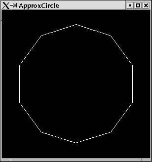
Example:
First we test what kind of shape we get for small approximation numbers.
ApproxCircle
import PointsForRendering
import Circle

import Graphics.Rendering.OpenGL

main = renderInWindow $ do
        clear [ColorBuffer]
        renderCircleApprox 0.8 10
The resulting graphic can be seen in figure 2.9.
Example:
Now we can test, if the resulting circle is, what we expected.
TestCircle
import PointsForRendering
import Circle

import Graphics.Rendering.OpenGL

main = renderInWindow $ do
          clear [ColorBuffer]
          renderCircle 0.8
The resulting graphic can be seen in figure 2.10.

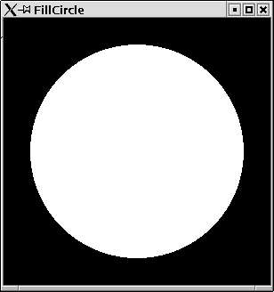
Example:
And eventually have a look at the filled circle.
FillCircle
import PointsForRendering
import Circle

import Graphics.Rendering.OpenGL

main
 = renderInWindow $ do
     clear [ColorBuffer]
     fillCircle 0.8
The resulting graphic can be seen in figure 2.11.
Rings
Now, where you know how to do circles, you can equally as easy define
functions for rendering rings. A ring has an inner and an outer circle
and fills the space between these. So we can approximate these two
rings and render quads between them.
Ring
module Ring where

import PointsForRendering
import Circle
import Graphics.Rendering.OpenGL
We can simply define the points of the inner and outer ring and merge
these. The resulting list of points can then be rendered as
a QuadStrip. Since there is no primitive mode for quad loops,
we need to append the first two points as the last points again:
Ring
ringPoints innerRadius outerRadius
 = concat$map (\(x,y)->[x,y]) (points++[p])
  where
    innerPoints = circle innerRadius
    outerPoints = circle outerRadius
    points@(p:_) = zip innerPoints outerPoints
Eventually we provide a small function for rendering ring shapes.
Ring
ring innerRadius outerRadius
 = displayPoints (ringPoints innerRadius outerRadius)  QuadStrip
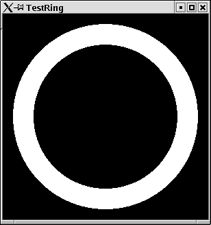
Example:
We can test the ring functions:
TestRing
import PointsForRendering
import Ring

import Graphics.Rendering.OpenGL

main = renderInWindow $  do
        clear [ColorBuffer]
        ring 0.7 0.9
The resulting graphic can be seen in figure 2.12.
2.2.4 Attributes of primitives
There are some more attributes that can be set for primitive shapes
(besides the color, which we have allready set).
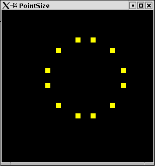
Point Size
You could argue that there is no need for single points. A point can
be modelled by a circle that has a small radius (or in the third
dimension a sphere). However, there is something like a point in
OpenGL and you can set its size. This size value for points does not
refer to a radius in the coordinate system but is measured in terms of
screen pixels. The default value is, one pixel per point.
Example:
We set the point size to 10 pixels:
PointSize
import Graphics.Rendering.OpenGL
import PointsForRendering

main = renderInWindow display

display = do
  pointSize $= 10
  displayMyPoints Points
The resulting graphic can be seen in figure 2.13.
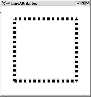
Line Attributes
As for points, there are also further attributes for lines. First of all
there is a line width. As for the point size, this is measured in
screen pixels. Furthermore, you can set some line stipple: this is the
pattern of the line, dashes etc. For the line stipple there is a
state variable of type: Maybe (GLint, GLushort). The second
argument of the value pair denotes the kind of stipple. For every
short value there is one stipple. The short value has 16 bits. Every
bit stands for a pixel. If for the corresponding short number the bit
is set, then the pixel will be drawn, otherwise not. This means that
for the short number 0 you will not see anything of your
line, and for the value 65535 you will see a solid line.
The integer number of the value pair denotes a factor for the chosen
stipple. For some positiv integer n every bit of the
short number stands for n bits.
Example:
Setting the width of lines and a stipple:
LineAttributes
import Graphics.Rendering.OpenGL
import Graphics.UI.GLUT  as GLUT
import PointsForRendering

main = renderInWindow display

display = do
  clearColor $= Color4 1 1 1 1
  clear [ColorBuffer]
  lineStipple $= Just (1,255)
  currentColor $= Color4 0 0 0 1
  lineWidth $= 10
  displayPoints squarePoints LineLoop
  flush

squarePoints
 = [(-0.7,-0.7,0),(0.7,-0.7,0),(0.7,0.7,0),(-0.7,0.7,0)]
The resulting graphic can be seen in figure 2.14.
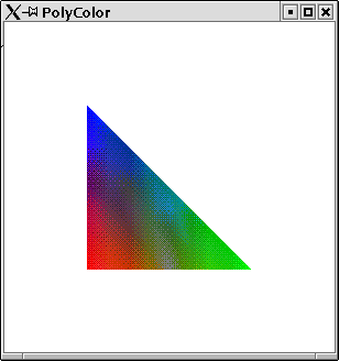
Colors
You might have wondered, why the function renderPrimitive takes monadic statements as argument and not
simply a list of vertexes? This means we could pass any monadic
statement to the function renderPrimitive, not only
statements that define vertexes by the call of the
function vertex. There are some statements, which are allowed
in the statements passed to renderPrimitive.
One of these is setting the current color before
every call of vertex to a new value. When finally rendering
the primitive, OpenGL takes these color values into acount.
Example:
We define a triangle. Before the three vertexes of the triangle are defined, the current color is set to a new value.
PolyColor
import Graphics.Rendering.OpenGL
import Graphics.UI.GLUT  as GLUT
import PointsForRendering

colorTriangle = do
  currentColor $= Color4 1 0 0 1
  vertex$Vertex3 (-0.5) (-0.5) (0::GLfloat)
  currentColor $= Color4 0 1 0 1
  vertex$Vertex3 (0.5) (-0.5) (0::GLfloat)
  currentColor $= Color4 0 0 1 1
  vertex$Vertex3 (-0.5) (0.5) (0::GLfloat)

main = renderInWindow display

display = do
  clearColor $= Color4 1 1 1 1
  clear [ColorBuffer]
  renderPrimitive Triangles colorTriangle
  flush
The resulting window can be found in figure 2.15.
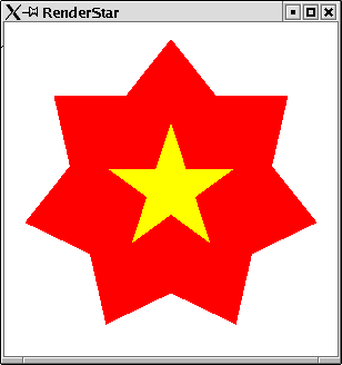
2.2.5 Tessellation
Rendering of polygons is very limited. We cannot render polygons for
crossing lines, or convex corners. Such polygons need to be expressed
by a set of simpler polygons.
In the module Graphics.Rendering.OpenGL.GLU.Tessellation there are a number of
functions, which calculate a set of simpler polygons.
For the time being, we will not go
into detail, but give one single example, of how to use this library.
Example:
We want to render stars. These are shapes with convex corners.
Star
module Star where
import Graphics.Rendering.OpenGL
import Graphics.UI.GLUT  as GLUT
import Data.Either
import Circle
import List
We can easily calculate the points on the star rays. They are all on
one circle. We can use our function for defining circle points and get
a list of points. For rendering the star, we take first the points
with odd index followed by the points with even index.
Star
starPoints radius rays
 = map (\(_,(x,y,z))->Vertex3 x y z)(os++es)
  where
   (os,es) = partition (\(i,_)-> odd i)
               $zip [1,2..]
               $circlePoints radius rays
For tesselation we need to create a ComplexPolygon, which has
a list of ComplexContour. A ComplexContour contains
a list of AnnotatedVertexes. The annotation can be used for
color or similar information. We do not make use of this annotation
and simple annotate every vertex with 0.
Star
complexPolygon points
 = ComplexPolygon
     [ComplexContour $map (\v->AnnotatedVertex v 0) points]
The function tesselate creates a list of simple polygons.
It needs some control information, which we do not explain here.
Star
star radius rays= do
  startess
    <- tessellate
         TessWindingPositive 0 (Normal3 0 0 0) noOpCombiner
            $complexPolygon (starPoints radius rays)
  drawSimplePolygon  startess
The resulting simple polygons can be rendered with the
function renderPrimitive.
Star
drawSimplePolygon  (SimplePolygon primitiveParts) =
  mapM_ renderPrimitiveParts primitiveParts

renderPrimitiveParts (Primitive primitiveMode vertices) =
  renderPrimitive primitiveMode
    $mapM_ (vertex . stripAnnotation) vertices

stripAnnotation (AnnotatedVertex plainVertex _) = plainVertex

noOpCombiner _newVertex _weightedProperties = 0.0 ::GLfloat
Now we can test our stars. We render two stars, one with 7 and one
with 5 rays.
RenderStar
import PointsForRendering
import Graphics.Rendering.OpenGL
import Graphics.UI.GLUT  as GLUT
import Star

main = renderInWindow$do
 clearColor $= Color4 1 1 1 1
 clear [ColorBuffer]

 currentColor $= Color4 1 0 0 1
 star 0.9 7

 currentColor $= Color4 1 1 0 1
 star 0.4 5
The resulting window can be found in figure 2.16.
2.2.6 Cubes, Dodecahedrons and Teapots
The bad news was that just very basic shapes are provided by OpenGL
for rendering. The good news is that the OpenGL library comes along
with a library that contains a large number of shapes.
Chapter 3
Example:
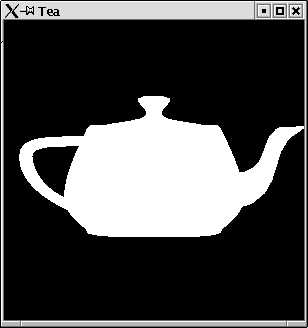
You probably need very often the shape of a teapot. Since this is so elementary a library function is provided for this.
Tea
import Graphics.UI.GLUT
import Graphics.Rendering.OpenGL

import PointsForRendering

main = renderInWindow display

display = do
  clear [ColorBuffer]
  renderObject Solid$ Teapot 0.6
  flush
The resulting graphic can be seen in figure 2.17.
Chapter 3
Modelling Transformations
By now you know, how to define different shapes for rendering. You
might wonder how to place shapes on special positions or how to
scale or rotate your shapes. This is done by so called transformation
matrixes. Before something is rendered by OpenGL a transformation
operation is performed on it. Every point will get multiplied with
the transformation matrix. The transformation matrix is part of the
state. So in order to transform a shape in some way, first the
transformation matrix has to be set and then the shapes are to be
rendered.
If not specified otherwise the transformation matrix is the identity
operation, i.e. no transformation is performed. You can
always reset the transformation matrix to the identity by the call of
the monadic statement loadIdentity. Then the current matrix
is discarded and no transformation is applied to the next rendering
operations.
3.1 Translate
One transformation is to move a shape to another position. The
according matrix is set by the statement translate. It has
one argument: a vector of size three which denotes in which direction
the following shapes are to be moved. Every vertex that will be
rendered after a translate statement will be moved by the
values of this vector.
Example:
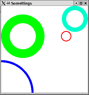
The function ring we defined before only defined rings which have the center coordinates (0,0,0). If we want to place rings somewhere else then we need to apply a translate matrix.
SomeRings
import PointsForRendering
import Ring
import Graphics.Rendering.OpenGL
We define a function, which creates a ring at a given
position. Therefore we first set the transformation to the
translate transformation then define the ring and finally set the
transformation matrix back to the identity:
SomeRings
ringAt x y innerRadius outerRadius = do
  translate$Vector3 x y (0::GLfloat)
  ring innerRadius outerRadius
We can test this by placing some ring in different colors on the screen.
SomeRings
main = do
  renderInWindow  someRings

someRings = do
  clearColor $= Color4 1 1 1 1
  clear [ColorBuffer]

  loadIdentity
  currentColor $= Color4 1 0 0 1
  ringAt 0.5 0.3 0.1 0.12

  loadIdentity
  currentColor $= Color4 0 1 0 1
  ringAt (-0.5) 0.3 0.3 0.5

  loadIdentity
  currentColor $= Color4 0 0 1 1
  ringAt (-1) (-1) 0.7 0.75

  loadIdentity
  currentColor $= Color4 0 1 1 1
  ringAt 0.7 0.7 0.2 0.3
The resulting graphic can be seen in figure 3.1.
Note that if we did not reset the transformation back to the identity,
we would get the composition of all transformations.
3.2 Rotate
Another transformation that can be performed is rotation. The rotate
statement has two arguments. The first one specifies by which degree
the following shapes are to be rotated counterclockwise. The second
argument is a vector which specifies around which axis the shape is
to be rotated.
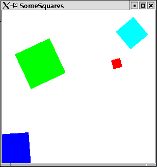
Example:
In this example we apply the composition of two transformations. Squares are moved to some position and furthermore rotated around the z-axis.
We write a simple module for rendering filled rectangles:
Squares
module Squares where

import Graphics.Rendering.OpenGL
import PointsForRendering
Here is a function for arbitrary rectangles:
Squares
myRect width height =
  displayPoints [(w,h,0),(w,-h,0),(-w,-h,0),(-w,h,0)] Quads
   where
     w = width/2
     h = height/2
A square is just a special case:
Squares
square width = myRect width width
Now we will transform squares.
SomeSquares
import PointsForRendering
import Squares
import Graphics.Rendering.OpenGL
We define a function, which applies the rotate transformation to a square. It is rotated around the z-axis.
SomeSquares
rotatedSquare alpha width  = do
  rotate alpha $Vector3 0 0 (1::GLfloat)
  square width
A further utility function moves some shape to a specified position. Note that this function resets the matrix again.
SomeSquares
displayAt x y displayMe = do
  translate$Vector3 x y (0::GLfloat)
  displayMe
  loadIdentity
Some squares are defined and rotated:
SomeSquares
main = do
  renderInWindow  someSquares

someSquares = do
  clearColor $= Color4 1 1 1 1
  clear [ColorBuffer]

  currentColor $= Color4 1 0 0 1
  displayAt 0.5 0.3$rotatedSquare  15 0.12

  currentColor $= Color4 0 1 0 1
  displayAt (-0.5) 0.3$rotatedSquare 25 0.5

  currentColor $= Color4 0 0 1 1
  displayAt (-1) (-1)$rotatedSquare 4 0.75

  currentColor $= Color4 0 1 1 1
  displayAt 0.7 0.7$rotatedSquare 40 0.3
The resulting graphic can be seen in figure 3.2.
3.3 Scaling
The third transformation enables you to scale shapes. This is not only
useful for changing the size of some object but for stretching it in
some direction. The transformation scale has three arguments,
which represent the scaling factors in the three dimensional space.
Remember that the scale and the rotate transformation always refer to
the origin (0,0,0) of your coordinates. Rotating an object,
which is not situated at the origin will move it around the
origin. Scaling an object which is not situated at the origin might
deform the object in surprising ways.
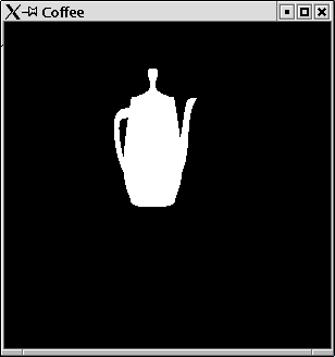
Example:
We apply three transformations on the tea pot example. We rotate and translate it and finally we stretch it a bit by a scale transformation.
Coffee
import Graphics.UI.GLUT
import Graphics.Rendering.OpenGL

import PointsForRendering
main = renderInWindow display

display = do
  clear [ColorBuffer]
  scale 0.3 0.9 (0.3::GLfloat)
  translate$Vector3 (-0.3) 0.3 (0::GLfloat)
  rotate 30 $Vector3 0 1 (0::GLfloat)
  renderObject Solid$ Teapot 0.6
  loadIdentity
  flush
The resulting graphic can be seen in figure 3.3. As you see it looks now like a coffee pot.
3.4 Composition of Transformations
Since Haskell is a functional programming language let us think of
transformations as functions. A transformation is a function that is
applied to every vertex before it is rendered. If you define two
transformations for an object, e.g. a rotation and a translation, then
you define a composition of these transformations.
The code:
rotatedSquareAt width alpha x y z = do
  translate$Vector3 x w y
  rotate alpha $Vector3 0 0 (1::GLfloat)
  square width
defines a composition of a translate und a rotate transformation, which is applied to a square figure. A sequence of transformation statements is composed to a single transformation in the same way as the standard function composition operator (.) composes functions: (f . g) x = f(g(x)). The compositional function (f . g) is the same as first applying function g and then applying f. For transformations in HOpenGL this means that for a sequence of transformations
translate$Vector3 x w y
rotate alpha $Vector3 0 0 (1::GLfloat)
first the points are rotated and then they are translated.
The order in which transformations are performed is of course not
arbitrary. A rotation after a translation is different to a
translation after a rotation.
Since the scale und the rotate transformation refer both to the origin
and the translate transformation can move objects away from the origin
it is a good policy to create objects at the origin, then rotate and
scale it and finally translate it to its final position. Therefore
predefined shapes in the library are usually positioned at the origin,
as e.g. the tea pot.
Example:
This example illustrates the different compositions of rotation and translation.
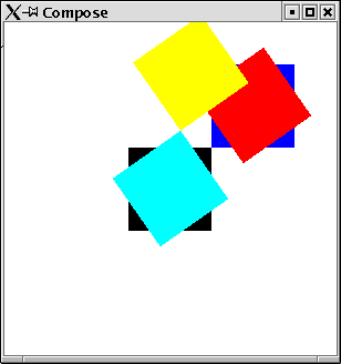
Compose
import PointsForRendering
import Squares
import Graphics.Rendering.OpenGL

displayAt x y displayMe = do
  displayMe
  loadIdentity

main = do
  renderInWindow  someSquares

someSquares = do
  clearColor $= Color4 1 1 1 1
  clear [ColorBuffer]
A black square at the origin:
Compose
  currentColor $= Color4 0 0 0 1
  square 0.5
  loadIdentity
A blue square translated:
Compose
  currentColor $= Color4 0 0 1 1
  translate$Vector3 0.5 0.5 (0::GLfloat)
  square 0.5
  loadIdentity
A light blue square that is rotated:
Compose
  currentColor $= Color4 0 1 1 1
  rotate 35 $Vector3 0 0 (1::GLfloat)
  square 0.5
  loadIdentity
A red square that is first rotated and then translated:
Compose
  currentColor $= Color4 1 0 0 1
  translate$Vector3 0.5 0.5 (0::GLfloat)
  rotate 35 $Vector3 0 0 (1::GLfloat)
  square 0.5
  loadIdentity
A yellow square that is first translated and then rotated:
Compose
  currentColor $= Color4 1 1 0 1
  rotate 35 $Vector3 0 0 (1::GLfloat)
  translate$Vector3 0.5 0.5 (0::GLfloat)
  square 0.5
  loadIdentity
The resulting window can be found in figure 3.4.
3.5 Defining your own transformation
The three ready to usee transformations rotation, scaling and
translation or their composition might not suffice for your
needs. Then you can define your own transformations. Technically a
transformation in OpenGL is represented as a matrix. Every vertex gets
multiplied by the transformation matrix before it is rendered. In
order to define a transformation, we will need to construct such a
matrix.
Internally every vertex in OpenGL is not represented by 3
coordinates (x,y,z) but by four
coordinates (x,y,z,w). The x, y, z values
are devided by w. Usually the value
of w is 1.0.
Thus for a transformation matrix you need a matrix of four rows and four
columns. Remember that a matrix is multiplied with a vector in the
following way:
|
OpenGL provides a function for creation of a transformation
matrix out of a list: matrix. It takes as first argument a
parameter, which specifies in which order the matrix elements appear
in the list: RowMajor for row wise and ColumMajor for column wise appearance. The function multMatrix allows to multiply your newly created transformation
matrix to the current transformation context.
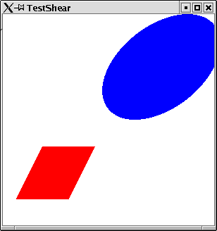
3.5.1 Shear
We can now define our own transformations. We can define the
transformation shear. Mathematical textbooks
define shear in the following way:
A transformation in which all points along a given
line L remain fixed while other points are shifted
parallel to L by a distance proportional to their
perpendicular distance from L.
Shearing a plane figure does not change its area.
Eric Weissteins's world of mathematics (http://mathworld.wolfram.com/Shear.html)
Eric Weissteins's world of mathematics (http://mathworld.wolfram.com/Shear.html)
We define a shear transformation, which leaves y and z coordinates unchanged, and adds to
the x coordinate some value depending on the value
of y. For some f we need the following
transformation matrix:
|
As you can see, this is almost the identity.
We can define this in HOpenGL:
MyTransformations
module MyTransformations where
import Graphics.Rendering.OpenGL
import Graphics.UI.GLUT  as GLUT

shear f = do
  m <-  (newMatrix RowMajor [1,f,0,0
                              ,0,1,0,0
                              ,0,0,1,0
                              ,0,0,0,1])
  multMatrix (m:: GLmatrix GLfloat)
Let us test our new transformation:
TestShear
import PointsForRendering
import Circle
import Squares
import MyTransformations

import Graphics.Rendering.OpenGL
import Graphics.UI.GLUT  as GLUT

main = renderInWindow$do
 loadIdentity
 clearColor $= Color4 1 1 1 1
 clear [ColorBuffer]
 translate$Vector3 0.5 0.5 (0::GLfloat)
 shear 0.5
 currentColor $= Color4 0 0 1 1
 fillCircle 0.5

 loadIdentity
 translate$Vector3 (-0.5) (-0.5) (0::GLfloat)
 shear 0.5
 currentColor $= Color4 1 0 0 1
 square 0.5
The resulting window can be found in figure 3.5.
3.6 Some Word of Warning
You might get strange effects when you forget to reset the
transformation matrix. This might not only effect further rendering
statements but also applies to the redisplay of your window. The display
function you specified for your window will be called whenever the
window needs to be displayed. However this does not automatically
reset the transformation matrix to the identity matrix. This results
in the effect that every redisplay of your window changes its contents.
Example:
In this example a ring is displayed. Each time the display function is called the contents of the ring moves a bit. Compile the program and hide the resulting window behind some other window. You will observe how the ring moves within the window, until it is no longer displayed.
ForgottenReset
import Graphics.UI.GLUT
import Graphics.Rendering.OpenGL

import PointsForRendering
import Ring
import Squares

main = renderInWindow display

display = do
  clear [ColorBuffer]
  translate$Vector3 (-0.1) 0.1 (0::GLfloat)
  ring 0.2 0.4
  flush
As a matter of fact this effect may not only occur with
transformations, but every state changing statement. If you set the
color as last statement in your display function to some value then
this will be the current color in the next call of the display
function. Thus it is better to ensure that the display function leaves
a clean state, i.e. the state it espects to find, when
it is called, or even better let the display functions
not rely on any previously set states.
3.7 Local transformations
Often you will have the situation, that you are in a context of some
transformations. Maybe for certain parts of you shape you want
to add some
further transformation but for other parts return to the outer
transformation context. In such situations you cannot use
the statement loadIdentity since this will not only delete
the transformations you wanted to be applied to your local part of the
the complete shape but the whole transformation context.
HOpenGL provides a function which allows to add some more
transformations to some local parts of your shape. This function is
called preservingMatrixs which refers to the fact that
transformations are technically implemented as
matrixes. preservingMatrix has one argument, which is a
monadic statement. The application of preservingMatrix is a
monadic statement:
preservingMatrix :: IO a -> IO aEvery transformation done within this monadic statement will not be done only locally. It does not effect the statements which follow after the application of preservingMatrix.
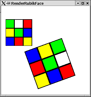
Example:
To demonstrate the use of preservingMatrix we provide a module, which is able to render a side of the famous Rubik's Cube. Such a side consists of 9 squares which are of some color and which have a black frame. We can render such a shape, by rendering the single framed squares at the origin and then move them to their position. This movement is done within a preservingMatrix application.
RubikFace
module RubikFace where
import Graphics.UI.GLUT
import Graphics.Rendering.OpenGL

import Squares
import PointsForRendering
Doing a frame involves the four sides of a frame. Each side is created at the origin and then moved to its final position:
RubikFace
frame width height border = do
  let bh = border/2
  let wh = width/2-bh
  let hh = height/2-bh

  preservingMatrix $ do
    translate $Vector3 0 hh (0::GLfloat)
    myRect width  border
  preservingMatrix $ do
    translate $Vector3 0 (-hh) (0::GLfloat)
    myRect width  border
  preservingMatrix $ do
    translate $Vector3 (-wh) 0 (0::GLfloat)
    myRect  border height
  preservingMatrix $ do
    translate $Vector3 wh 0 (0::GLfloat)
    myRect  border height
Each of the nine fields is rendered by drawing its frame and its
colored square:
RubikFace
originField width color = do
  let frameWidth = width/10
  currentColor $= Color4 0 0 0 1
  frame width width frameWidth
  let sc = 18/20::GLfloat
  currentColor $= color
  square (width-frameWidth)
Eventually the side of Rubik's Cube can be drawn
RubikFace
renderArea :: GLfloat -> [[Color4 GLfloat]] -> IO ()
renderArea width css
 = do
    let cs  = concat css
        cps = zip cs $ areaFields width
    mapM_  (\(c,f)-> f(originField width c)) cps

areaFields width =
  [makeSquare x y |x<-[1,0,-1],y<-[1,0,-1]]
    where
      makeSquare xn yn = \f -> preservingMatrix $ do
       let
         x = xn*width
         y = yn*width
       translate $Vector3 x y 0
       f

red     = Color4 1 0 0 (1::GLfloat)
green   = Color4 0 1 0 (1::GLfloat)
blue    = Color4 0 0 1 (1::GLfloat)
yellow  = Color4 1 1 0 (1::GLfloat)
white   = Color4 1 1 1 (1::GLfloat)
black   = Color4 0 0 0 (1::GLfloat)
The following module tests the rendering. Two sides are
rendered. Further transformations are applied to them.
RenderRubikFace
import PointsForRendering
import Graphics.Rendering.OpenGL

import PointsForRendering
import RubikFace

_FIELD_WIDTH :: GLfloat
_FIELD_WIDTH = 1/5

main =  renderInWindow  faces

faces = do
  clearColor $= white
  clear [ColorBuffer]

  loadIdentity
  translate  $Vector3 (-0.6) 0.4 (0::GLfloat)
  renderArea _FIELD_WIDTH r1

  loadIdentity
  translate  $Vector3 (0.1) (-0.3) (0::GLfloat)
  rotate 290 $ Vector3 0 0 (1::GLfloat)
  scale 1.5 1.5 (1::GLfloat)
  renderArea _FIELD_WIDTH r1

r1=[[red,blue,yellow],[white,green,red],[green,yellow,blue]]
The resulting window can be found in figure 3.6.
Chapter 4
Projection
4.1 The Function Reshape
Up to now we always relied on the default values for most attributes
which are concerned with projection. From where do we look at the
scenery? Which coordinates are displayed to what extend on the
screen. Such attributes can be set in the reshape callback
function. This function gets the window size as argument and specifies
which coordinates are to be seen on the screen. At first glance the
name seems to be a bit misleading, since it evokes the image that it is
just called, when someone resizes the window. The first time the
reshape function is called is at the opening of the window.
The reshape function might be empty. This is modelled by the Haskell
data type Maybe.
Example:
We define the first reshape function for a window. It is the identity function, which does not specify anything, how to render the picture.
Reshape1
import Graphics.UI.GLUT
import Graphics.Rendering.OpenGL

import PointsForRendering

main = do
  (progName,_) <- getArgsAndInitialize
  createWindow progName
  displayCallback $= display
  reshapeCallback $= Just reshape
  mainLoop

display = do
 clear [ColorBuffer]
 displayPoints points Quads
   where
    points
     = [(0.5,0.5,0)
       ,(-0.5,0.5,0)
       ,(-0.5,-0.5,0)
       ,(0.5,-0.5,0)]

reshape s = return ()
Run this example. You will see a white square in the middle of a black
screen. Now resize the window. You will notice that the size of the
square will not change. If you make the window smaller parts of the
picture are not displayed, if you enlarge the window parts of the
window contain no image (which means it might be some arbitrary
image). Figure 4.1 shows how the window looks after enlarging
it a bit.
4.2 Viewport: The Visible Part of Screen
Usually you want to define in the reshape function, which parts of the
window pane are to be used for rendering the picture. There is a state
variable viewport, which contains exactly this
information. It is a pair, of a position and a size. The position is
the offset from the upper left corner in pixels. The size is the size
of the screen to be used for rendering in pixels.
Example:
If you want the window to be used completely for rendering the image, then the position needs to be set to Position 0 0. i.e. no offset and as size the complete window size is to be used:
Reshape2
import Graphics.UI.GLUT
import Graphics.Rendering.OpenGL

import PointsForRendering

main = do
  (progName,_) <- getArgsAndInitialize
  createWindow progName
  displayCallback $= display
  reshapeCallback $= Just reshape
  mainLoop

display = do
  clear [ColorBuffer]
  displayPoints points Quads
   where
    points
     = [(0.5,0.5,0)
       ,(-0.5,0.5,0)
       ,(-0.5,-0.5,0)
       ,(0.5,-0.5,0)]

reshape s@(Size w h) = do
  viewport $= (Position 0 0, s)
If you start this program and resize the window, then always the
complete window pane will be used for rendering your image.
Example:
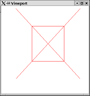
In this example only parts of the window are used for rendering the image. The image is smaller than the window.
Viewport
import Graphics.UI.GLUT
import Graphics.Rendering.OpenGL

import PointsForRendering

main = do
  (progName,_) <- getArgsAndInitialize
  createWindow progName
  clearColor $= Color4 0 0 0 0
  displayCallback $= display
  reshapeCallback $= Just reshape
  mainLoop

display = do
  clearColor $= Color4 1 1 1 1
  clear [ColorBuffer]
  currentColor $= Color4 1 0 0 1
  displayPoints ps1 LineLoop
  displayPoints ps2 Lines
   where
    ps1=[(0.5,0.5,0),(-0.5,0.5,0),(-0.5,-0.5,0),(0.5,-0.5,0)]
    ps2=[(1,1,0),(-1,-1,0),(-1,1,0),(1,-1,0) ]

reshape s@(Size w h) = do
  viewport $= (Position 50 50, Size (w-80) (h-60))
The resulting window can be found in figure 4.2.
4.3 Orthographic Projection
The viewport defines which parts of your window pane are used for
rendering your image. The actual projection defines which coordinates
you want to display. The simpliest way to specify this is by the
function ortho. It has six arguments, the lower and upper
bounds of the x, y, z coordinates.
Projection is equally as transformation internally expressed in terms
of a matrix. The statement loadIdentity can refer to the
transformation or to the projection matrix. A state variabble matrixMode defines, which of these matrixes these statements
refer to. Therefore it is necessary to switch this variable to the
value Projection, before applying the function ortho and afterwards to reset the variable back to the
value ModelView.
ortho is the simpliest projection we can define. When we will
consider third dimensional szeneries we will learn a more powerful
projection.
Chapter 5
Example:
We render the same image in two windows with different projection values:
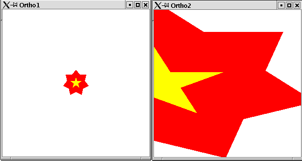
Ortho
import PointsForRendering
import Graphics.Rendering.OpenGL
import Graphics.UI.GLUT  as GLUT
import Star

main = do
  (progName,_) <-  getArgsAndInitialize

  createWindow (progName++"1")
  displayCallback $= display
  projection (-5) 5 (-5) 5 (-5) 5

  createWindow (progName++"2")
  displayCallback $= display
  projection 0 0.8 (-0.8) 0.8 (-0.5) 0.5

  mainLoop

projection xl xu yl yu zl zu = do
  matrixMode $= Projection
  loadIdentity
  ortho xl xu yl yu zl zu
  matrixMode $= Modelview 0

display = do
 clearColor $= Color4 1 1 1 1
 clear [ColorBuffer]
 currentColor $= Color4 1 0 0 1
 star 0.9 7
 currentColor $= Color4 1 1 0 1
 star 0.4 5
The resulting windows can be found in figure 4.3.
Chapter 5
Changing States
OpenGL is not only designed to render static images, but to have
changing images. There are to ways how your image might change:
- it might react to some event, like some keyboard input or mouse event.
- it might change over time.
In order to change your image in some coordinated way, you need a
state which can change. An event may change your state, or over the time
your state might be changed.
5.1 Modelling your own State
A state is of course something, which does not match the purely
functional paradigm of Haskell. However in the context of I/O the
designers of Haskell came up with some clever way to integrate state changing
variables into the Haskell's purely functional setting. The trick are
again monads, as you have seen before for the state machine of
OpenGL. There is a standard library in Haskell for state changing
variables: Data.IORef. This provides functions for creation,
setting, retrieving and modification of state variables. These functions are
called:
newIORef, writeIORef, readIORef, modifyIORef.
newIORef, writeIORef, readIORef, modifyIORef.
If you think these names a bit too technical, then you might use the
following module, which makes IORef variables instances of
the type classes HasGetter and HasSetter. Thus we
can use our own state variables in the same way, we use the HOpenGL
state variables.7
StateUtil
module StateUtil where

import Graphics.Rendering.OpenGL
import Data.IORef
import Graphics.UI.GLUT

--instance HasSetter IORef  where
--  ($=) var val = writeIORef var val

--instance HasGetter IORef  where
--  get var = readIORef var

new = newIORef
5.2 Handling of Events
Now we know how to modell our own state. We can use this for reacting
on some events. Event handling in HOpenGL is done by setting a
callback function for mouse and keyboard events.
A callback function for mouse and keyboard events needs to be of the
following type:
type KeyboardMouseCallback =
   Key -> KeyState -> Modifiers -> Position -> IO ()
A Key can be some character, some special character or some
mouse buttom:
data Key
   = Char Char
   | SpecialKey SpecialKey
   | MouseButton MouseButton
   deriving ( Eq, Ord, Show )
The keystate informs, if the key has been pressed or released.
data KeyState
   = Down
   | Up
   deriving ( Eq, Ord, Show )
A modifier denotes, if some extra key is used, like the alt, strg or
shift key:
data Modifiers = Modifiers { shift, ctrl, alt :: KeyState }
   deriving ( Eq, Ord, Show )
And finally the position informs about the current mouse pointer
position.
5.2.1 Keyboard events
With the close look at the event handling function above it is fairly
easy to write a program that reacts on keyboard events. A function of
type KeyboardMouseCallback is to be written and assigned to
the state variable keyboardMouseCallback of your
window. Usually your KeyboardMouseCallback will have access
to some of your state variables, since you want to change a state when
an event occurs. When the state has been changed, HOpenGL needs to be
forced to redisplay the picture with the new state values. Therefore a
call to the function postRedisplay needs to be done.
Example:
In this example we draw a circle. The radius of the circle can be changed by use of the + and - key.
State
import Circle
import PointsForRendering
import StateUtil

import Graphics.Rendering.OpenGL
import Data.IORef
import Graphics.UI.GLUT

main = do
  (progName,_) <-  getArgsAndInitialize
  createWindow progName
We create a state variable which stores the current radius of the circle:
State
radius <- new 0.1
The display function gets this state variable as first argument:
State
displayCallback $= display radius
And the keyboard callback gets this variable as first argument:
State
  keyboardMouseCallback $= Just (keyboard radius)
  mainLoop
The display function gets the current value for the radius and draws a
filled circle:
State
display radius = do
  clear [ColorBuffer]
  r <- get radius
  fillCircle r
The keyboard callback reacts on two keyboard events. The value of the
radius variable are changed:
State
keyboard radius (Char '+') Down _ _ = do
  r <- get radius
  radius $=  r+0.05
  postRedisplay Nothing
keyboard radius (Char '-') Down _ _ = do
  r <- get radius
  radius $=  r-0.05
  postRedisplay Nothing
keyboard _ _ _ _ _ = return ()
Compile and start this program and press the + and - key.
5.3 Changing State over Time
The second way to change your picture is over time. You can create an
animation if your picture changes a tiny bit every moment. In HOpenGL
you can a define a so called idle function. This function
will be evaluated whenever the picture has been displayed. There you
can define, in what way your state will change before the next
redisplay is performed. The last statement in an idle function will be
usually a call to postRedisplay.
Example:
We define our first animation. A ring is displayed with a changing radius.
Idle
import Ring
import PointsForRendering
import StateUtil

import Graphics.Rendering.OpenGL
import Data.IORef
import Graphics.UI.GLUT  as GLUT
We define a constant which denotes the value by which the radius changes between every redisplay:
Idle
_STEP = 0.001Within the main function an idle callback is added to the window:
Idle
main = do
  (progName,_) <-  getArgsAndInitialize
  createWindow progName
  radius <- new 0.1
  step   <- new _STEP
  displayCallback $= display radius
  idleCallback $= Just (idle radius step)
  mainLoop
The display function renders a ring, depending on the state variable for the radius:
Idle
display radius = do
  clear [ColorBuffer]
  r <- get radius
  ring r (r+0.2)
  flush
The idle function changes the value of the variable radius depending on the second state variable step.
Idle
idle radius step = do
  r <- get radius
  s <- get step
  if r>=1 then step $= (-_STEP)
          else if r<=0 then step $= _STEP
                       else return ()
  s <- get step
  radius $= r+s
  postRedisplay Nothing
5.3.1 Double buffering
The animation created in the last example was not very satisfactory. A
ring with changing radius was displayed, but the animation was somehow
flickering. The reason for that was, that the display function as its
first statement clears the screen, i.e. makes it alltogether
black. Only afterwards the ring is rendered. For a short moment the
screen will be completely black. This is what makes this flickering
effect.
A common solution for this problem in animated pictures is, not to
apply the statements of the display function directly to the screen,
but to an invisible buffer. When all statements of the display
function have been applied to this invisible background buffer, this
buffer is copied to the screen. This way only the ready to use final
picture is shown on screen and not any intermediate rendering step
(e.g. the picture after the clear statement).
OpenGL provides a double buffering mechanism. We only have to activate
this. Therefore we need to set the initial display mode variable
accordingly. Instead of a call to the function flush a call
to the function swapBuffers needs to be done as last
statement of the display function.
Example:
The ring with changing radius over time now with double buffering.
Double
import Ring
import PointsForRendering
import StateUtil

import Graphics.Rendering.OpenGL
import Data.IORef
import Graphics.UI.GLUT  as GLUT

_STEP = 0.001

main = do
  (progName,_) <-  getArgsAndInitialize
  initialDisplayMode $= [DoubleBuffered]
  createWindow progName
  radius <- new 0.1
  step   <- new _STEP
  displayCallback $= display radius
  idleCallback $= Just (idle radius step)
  mainLoop

display radius = do
  clear [ColorBuffer]
  r <- get radius
  ring r (r+0.2)
  swapBuffers

idle radius step = do
  r <- get radius
  s <- get step
  if r>=1 then step $= (-_STEP)
          else if r<=0 then step $= _STEP
                       else return ()
  s <- get step
  radius $= r+s
  postRedisplay Nothing
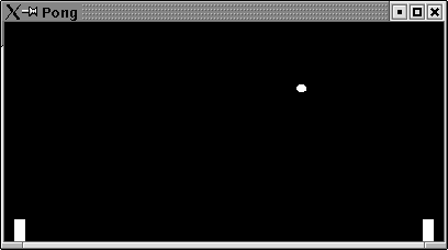
5.4 Pong: A first Game
By now you have seen a lot of tiny examples. It is time to draw the
techniques together and do an application with HOpenGL. In this
section we will implement one of the first animated computer games
ever: Pong. It consists of a small white circle which moves
over a black screen and two paddles which can move on a vertical line.
Pong in action can be found in figure 5.1.
Pong
import Circle
import Squares
import PointsForRendering
import StateUtil

import Graphics.Rendering.OpenGL
import Data.IORef
import Graphics.UI.GLUT  as GLUT
First of all we define some constant values for the game:
x-, y-coordinates of the game, width and height of a paddle, the
radius of the ball, initial factor, how a ball and a paddle changes
its position, and an initial board size.
Pong
_LEFT  = -2
_RIGHT =  1
_TOP   =  1
_BOTTOM= -1

paddleWidth  = 0.07
paddleHeight = 0.2
ballRadius   = 0.035

_INITIAL_WIDTH :: GLsizei
_INITIAL_WIDTH=400

_INITIAL_HEIGHT::GLsizei
_INITIAL_HEIGHT=200

_INITIAL_BALL_DIR = 0.002
_INITIAL_PADDLE_DIR = 0.005
We define a data type, game. The game state can be characterized by the position of the ball and the values these coordinates change for the next redisplay:
Pong
data Ball = Ball (GLfloat,GLfloat) GLfloat GLfloat
The paddles, which are characterized by their position and the
position change on the y-axis (x-axis is fixed for a paddle).
Pong
type Paddle = (GLfloat,GLfloat,GLfloat)
Additionally a game has points for the left and the right player and a
factor which denotes how fast ball and paddles move:
Pong
data Game
 = Game { ball ::Ball
        , leftP,rightP :: Paddle
        , points ::(Int,Int)
        , moveFactor::GLfloat}
For a starting game we provide the following initial game state:
Pong
initGame
 = Game {ball=Ball (-0.8,0.3) _INITIAL_BALL_DIR _INITIAL_BALL_DIR
        ,leftP=(_LEFT+paddleWidth,_BOTTOM,0)
        ,rightP=(_RIGHT-2*paddleWidth,_BOTTOM,0)
        ,points=(0,0)
        ,moveFactor=1
        }
The main function creates a double buffering window in fullscreen
mode. An initial game state is created and passed to the keyboard,
display, idle and reshape function:
Pong
main = do
  (progName,_) <-  getArgsAndInitialize
  initialDisplayMode $= [DoubleBuffered]
  createWindow progName
  game <- newIORef initGame
  --windowSize $= Size _INITIAL_WIDTH _INITIAL_HEIGHT
  fullScreen
  displayCallback $= display game
  idleCallback $= Just (idle game)
  keyboardMouseCallback $= Just (keyboard game)
  reshapeCallback $= Just (reshape game)
  mainLoop
The display function simply gets the ball and paddles from the game
state and renders these:
Pong
display game = do
  clear [ColorBuffer]
  g <- get game
  let (Ball  pos xDir yDir) = ball g
  --a ball is a circle
  displayAt pos $ fillCircle ballRadius
  displayPaddle$leftP g
  displayPaddle$rightP g
  swapBuffers
Paddles are simply rectangles:
Pong
displayPaddle (x,y,_) =  preservingMatrix$do
  translate$Vector3 (paddleWidth/2) (paddleHeight/2) 0
  displayAt (x,y)$myRect paddleWidth paddleHeight
We made use of the utility function which moves a shape to some position:
Pong
displayAt (x, y) displayMe = preservingMatrix$do
  translate$Vector3 x y (0::GLfloat)
  displayMe
Within the idle function ball and paddles need to be set to their next
position on the field:
Pong
idle game = do
  g <- get game
  let fac = moveFactor g
  game
    $= g{ball   = moveBall g
        ,leftP  = movePaddle (leftP g) fac
        ,rightP = movePaddle (rightP g) fac
        }
  postRedisplay Nothing
The movement on the ball is determined by the upper and lower bound of
the field, by the left and right bound of the field and the position
of the paddles:
Pong
moveBall g
 = Ball (x+factor*newXDir,y+factor*newYDir) newXDir newYDir
  where
   newXDir
    |      x-ballRadius <= xl+paddleWidth
       &&  y+ballRadius >=yl
       &&  y            <=yl+paddleHeight
       = -xDir
    |x <= _LEFT-ballRadius = 0
    |     x+ballRadius >= xr
       &&  y+ballRadius >=yr
       &&  y            <=yr+paddleHeight
       = -xDir
    |x >= _RIGHT+ballRadius = 0
    |otherwise    = xDir
   newYDir
    |y > _TOP-ballRadius || y< _BOTTOM+ballRadius = -yDir
    |newXDir == 0 = 0
    |otherwise = yDir
   (Ball (x,y) xDir yDir) = ball g
   factor = moveFactor g
   (xl,yl,_) = leftP g
   (xr,yr,_) = rightP g
A paddle moves only on the y-axis. We just need to ensure that it
does not leaves the field. There are maximum and minimum values for y:
Pong
movePaddle (x,y,dir) factor =
  let y1 = y+ factor*dir
      newY = min  (_TOP-paddleHeight) $max _BOTTOM y1
  in (x,newY,dir)
The keyboard function: key 'a' moves the left paddle, key 'l' the
right paddle and the space key gets a new ball:
Pong
keyboard game (Char 'a') upDown _ _ = do
  g <- get game
  let (x,y,_) = leftP g
  game $= g{leftP=(x,y,paddleDir upDown)}
keyboard game (Char 'l') upDown _ _ = do
  g <- get game
  let (x,y,_) = rightP g
  game $= g{rightP=(x,y,paddleDir upDown)}
keyboard game (Char '\32') Down _ _ = do
  g <- get game
  let Ball (x,y) xD yD = ball g
  let xDir
       |x<=_LEFT+3*paddleWidth = _INITIAL_BALL_DIR
       |x>=_RIGHT-3*paddleWidth = - _INITIAL_BALL_DIR
       |otherwise = xD
  if (xD==0)
    then game$=g{ball=Ball (x+4*xDir,y) xDir _INITIAL_BALL_DIR}
    else return ()
keyboard _ _ _ _ _ = return ()

paddleDir Down = _INITIAL_PADDLE_DIR
paddleDir Up   = -_INITIAL_PADDLE_DIR
Finally we define the visual part of the screen. The movement factor
of the ball depends on the width of the screen:
Pong
reshape game s@(Size w h)  = do
  viewport $= (Position 0 0, s)
  matrixMode $= Projection
  loadIdentity
  ortho (-2.0) 1.0 (-1.0) 1.0 (-1.0) 1.0
  matrixMode $= Modelview 0
  g <- get game
  game$=g{moveFactor=fromIntegral w/fromIntegral _INITIAL_WIDTH}
Have a break and play Pong.
Chapter 6
Chapter 6
Third Dimension
Up to now everything was pretty boring. We never considered the three
dimensional space provided by OpenGL. Strictly we just considered two
dimensions. Thus the library was not any more powerfull than any
simple graphics libaray e.g. like Java's java.awt.Graphics class. In this chapter we will explore the
true power of OpenGL by actually rendering three dimensional objects.
6.1 Hidden Shapes
In a three dimensional space some objects will be in front of others
and hide them. We would expect to see only those areas which are not
hidden by areas closer to the viewer.
By default OpenGL does not take the depth into account. Shapes
rendered later hide
other shapes which were rendered earlier, neglecting the depth of the
shapes. OpenGL provides a mechanism for automatically considering the
depth of a shape. This simply needs to be activated.
Three steps need to be done:
Example:
We render two shapes. A red square which is closer to the viewer and a blue circle which is farer away:
NotHidden
import Graphics.Rendering.OpenGL
import Graphics.UI.GLUT  as GLUT
import Squares
import Circle
import PointsForRendering

main = do
  (progName,_) <-  getArgsAndInitialize
  createWindow progName
  displayCallback $= display
  clearColor $= Color4 1 1 1 1
  mainLoop

display = do
  clear [ColorBuffer,DepthBuffer]
  loadIdentity
  translate (Vector3 0 0 (-0.5::GLfloat))
  currentColor $= Color4 1 0 0 1
  square 1

  loadIdentity
  translate (Vector3 0.2 0.2 (0.5::GLfloat))
  currentColor $= Color4 0 0 1 1
  fillCircle 0.5
  flush
However as can be seen in figure 6.1, the blue circle hides parts of the red square.
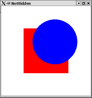
- as initial display mode WithDepthBuffer needs to be set.
- a depth function needs to be set. Usually the Less mode is used as function here. This ensures that closer objects hide objects farer away.
- the depth buffer needs to be cleared in the beginning of the display function.
Example:
Now we render the same to shapes as in the example before, but the depth machanism of OpenGL is activated.
Hidden
import Graphics.Rendering.OpenGL
import Graphics.UI.GLUT  as GLUT

import Squares
import Circle
import PointsForRendering

main = do
  (progName,_) <-  getArgsAndInitialize
  initialDisplayMode $= [WithDepthBuffer]

  createWindow progName

  depthFunc $= Just Less
  displayCallback $= display
  clearColor $= Color4 1 1 1 1
  mainLoop

display = do
  clear [ColorBuffer,DepthBuffer]
  loadIdentity
  translate (Vector3 0 0 (-0.5::GLfloat))
  currentColor $= Color4 1 0 0 1
  square 1

  loadIdentity
  translate (Vector3 0.2 0.2 (0.5::GLfloat))
  currentColor $= Color4 0 0 1 1
  fillCircle 0.5
  flush
Now as can be seen in figure 6.2, the
red square hides parts of the blue circle.
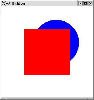
6.2 Perspective Projection
In the real world objects closer to the viewer appear larger than
objects farer away from the viewer. Up to now we only learnt how to
set up an orthographic projection. In an orthographic projection
objects farer away have the same size as object close to the viewer.
OpenGL provides the function frustum for specifying a
perspective projection. frustum has 6 arguments:
Example:
We can test the orthographic projection. Two squares equally in size, but in different distances from the viewer are rendered:
NotSmaller
import Graphics.Rendering.OpenGL
import Graphics.UI.GLUT  as GLUT

import Squares
import Circle
import PointsForRendering

main = do
  (progName,_) <-  getArgsAndInitialize
  initialDisplayMode $= [WithDepthBuffer]
  createWindow progName
  depthFunc $= Just Less
  displayCallback $= display

  matrixMode $= Projection
  loadIdentity
  ortho (-5) 5  (-5) 5 (1) 40
  matrixMode $= Modelview 0

  clearColor $= Color4 1 1 1 1
  mainLoop

display = do
  clear [ColorBuffer,DepthBuffer]
  loadIdentity
  translate (Vector3 0 0 (-2::GLfloat))
  currentColor $= Color4 1 0 0 1
  square 1

  loadIdentity
  translate (Vector3 4 4 (-5::GLfloat))
  currentColor $= Color4 0 0 1 1
  square 1
  flush
As can be seen in figure 6.3 , the
two squares have the same size, even though the red one is closer to
the viewer.
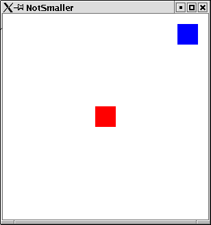
- left: left bound for the closest orthogonal plane
- right: right bound for the closest orthogonal plane
- top: upper bound for the closest orthogonal plane
- bottom: lower bound for the closest orthogonal plane
- near: the closest things that can be seen
- far: the farest away things that can be seen
Figure 6.4 illustrates these six values.
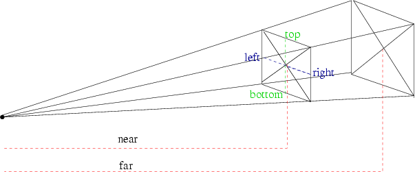
Usually you will have negated values for top/botton and left/right.
HopenGL provides a second function to define a perspective
projection: perspective. Here instead of left, right, top,
bottom an angle between the top/bottom ray and the width of the
closest plane can be specified.
Example:
Now we render the two squares from the previous example again. This time we use a perspective projection:
Smaller
import Graphics.Rendering.OpenGL
import Graphics.UI.GLUT  as GLUT

import Squares
import Circle
import PointsForRendering

main = do
  (progName,_) <-  getArgsAndInitialize
  initialDisplayMode $= [WithDepthBuffer]
  createWindow progName
  depthFunc $= Just Less
  displayCallback $= display

  matrixMode $= Projection
  loadIdentity
  let near   = 1
      far    = 40
      right  = 1
      top    = 1
  frustum (-right) right (-top) top near far
  matrixMode $= Modelview 0

  clearColor $= Color4 1 1 1 1
  mainLoop

display = do
  clear [ColorBuffer,DepthBuffer]
  loadIdentity
  translate (Vector3 0 0 (-2::GLfloat))
  currentColor $= Color4 1 0 0 1
  square 1

  loadIdentity
  translate (Vector3 4 4 (-5::GLfloat))
  currentColor $= Color4 0 0 1 1
  square 1
  flush
Now, as can be seen in figure 6.5, the
blue square appears to be smaller than the red square.
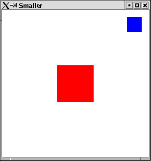
Figure 6.6 illustrates these values.
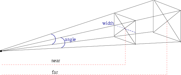
6.3 Setting up the Point of View
In the previous section we have learnt that there is a second way how
to project the three dimensional space onto the two dimensional area
of the screen. We did however not yet specify, where in the three
dimensional space the viewer is situated and in what direction they
are looking. In order to define this, OpenGL provides the
function lookAt. It has three arguments:
- the point, where the viewer is situated.
- the point at which the viewer is looking.
- and a vector, which specifies the direction which is to be up for the viewer.
6.3.1 Oribiting around the origin
The point of view, where we are looking from is interesting, when we
change it. In the following a module is defined, which allows
the viewer to move along a sphere. The
point of view can be set for a given sphere position. The position is
specified by two angles and a radius. The first angle defines which
way to move around the x-axis the second angle, which angle to move
around the y-axis. The radius defines the distance from the origin.
The position can be changed through keyboard events.
OrbitPointOfView
module OrbitPointOfView where

import Graphics.Rendering.OpenGL
import Graphics.UI.GLUT  as GLUT

import StateUtil
import Data.IORef

setPointOfView pPos = do
  (alpha,beta,r) <- get pPos
  let
   (x,y,z)    = calculatePointOfView alpha beta r
   (x2,y2,z2) = calculatePointOfView ((alpha+90)`mod` 360) beta r
  lookAt (Vertex3 x y z) (Vertex3 0 0 0) (Vector3 x2 y2 z2)

calculatePointOfView  alp bet r =
  let alpha =  fromIntegral alp*2*pi/fromIntegral 360
      beta  =  fromIntegral bet*2*pi/fromIntegral 360
      y = r * cos alpha
      u = r * sin alpha
      x = u * cos beta
      z = u * sin beta
  in (x,y,z)

keyForPos pPos (Char '+')         = modPos pPos (id,id,\x->x-0.1)
keyForPos pPos (Char '-')         = modPos pPos (id,id,(+)0.1)
keyForPos pPos (SpecialKey KeyLeft) = modPos pPos (id,(+)359,id)
keyForPos pPos (SpecialKey KeyRight)= modPos pPos (id,(+)1,id)
keyForPos pPos (SpecialKey KeyUp)   = modPos pPos ((+)1,id,id)
keyForPos pPos (SpecialKey KeyDown) = modPos pPos ((+)359,id,id)
keyForPos  _  _                     = return ()

modPos pPos (ffst,fsnd,ftrd) = do
  (alpha,beta,r) <- get pPos
  pPos $= (ffst alpha `mod` 360,fsnd beta `mod` 360,ftrd r)
  postRedisplay Nothing

reshape screenSize@(Size w h) = do
  viewport $= ((Position 0 0), screenSize)
  matrixMode $= Projection
  loadIdentity
  let near   = 0.001
      far    = 40
      fov    = 90
      ang    = (fov*pi)/(360)
      top    = near / ( cos(ang) / sin(ang) )
      aspect = fromIntegral(w)/fromIntegral(h)
      right = top*aspect
  frustum (-right) right (-top) top near far
  matrixMode $= Modelview 0
Example:
Let us use the module above, to orbit around a cube. Therefore we a define simple module, which renders a cube with differently colored areas. The cube is situated at the origin. We render the six areas by rendering a square at the origin and translate and rotate it into its final position.
ColorCube
module ColorCube where

import Graphics.Rendering.OpenGL
import Graphics.UI.GLUT  as GLUT

import Squares
import StateUtil

locally = preservingMatrix

colorCube n = do
  locally $ do
    currentColor $= Color4 1 0 0 1
    translate$Vector3 0 0 (-n/2)
    square n
  locally $ do
    currentColor $= Color4 0 1 0 1
    translate$Vector3 0 0 (n/2)
    square n
  locally $ do
    currentColor $= Color4 0 0 1 1
    translate$Vector3 (n/2) 0 0
    rotate 90 $Vector3 0 (1::GLfloat) 0
    square n
  locally $ do
    currentColor $= Color4 1 1 0 1
    translate$Vector3 (-n/2) 0 0
    rotate 90 $Vector3 0 (1::GLfloat) 0
    square n
  locally $ do
    currentColor $= Color4 0 1 1 1
    translate$Vector3 0 (-n/2) 0
    rotate 90 $Vector3 (1::GLfloat) 0 0
    square n
  locally $ do
    currentColor $= Color4 1 1 1 1
    translate$Vector3 0 (n/2) 0
    rotate 90 $Vector3 (1::GLfloat) 0 0
    square n
The following program allows to use the cursor keys to move around a
cube at the origin:
OrbitAroundCube
import Graphics.Rendering.OpenGL
import Graphics.UI.GLUT  as GLUT

import Squares
import OrbitPointOfView
import StateUtil
import ColorCube

main = do
  (progName,_) <-  getArgsAndInitialize
  initialDisplayMode $= [WithDepthBuffer,DoubleBuffered]
  createWindow progName
  depthFunc $= Just Less

  pPos <- new (90::Int,270::Int,2.0)
  keyboardMouseCallback $= Just (keyboard pPos)

  displayCallback $= display pPos
  reshapeCallback $= Just reshape
  mainLoop
The display function sets the viewer's position before rendering the
cube:
OrbitAroundCube
display pPos = do
  loadIdentity
  setPointOfView pPos
  clear [ColorBuffer,DepthBuffer]
  colorCube 1
  swapBuffers
As keyboard function we map directly to the function defined
in OrbitPointOfView.
OrbitAroundCube
keyboard pPos c _ _ _ = keyForPos pPos c
An example how the colored cube can now be seen
is given in figure 6.7.
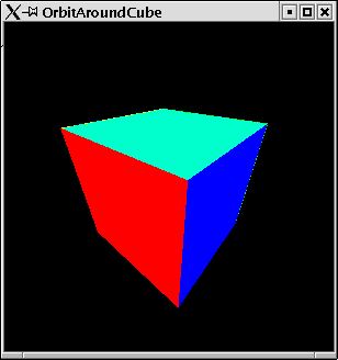
6.4 3D Game: Rubik's Cube
In this section we implement a primitive version of Rubik's cube.
Rubik's cube in action can be found in figure 6.8.
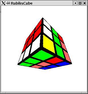
6.4.1 Cube Logics
First of all we modell the logics of Rubic's Cube8.
A data type is provided for representation of a cube:
RubikLogic
module RubikLogic where

data Rubik a
 = Rubik (Front a) (Top a) (Back a) (Bottom a) (Left a) (Right a)

type Front a  = Area a
type Top a    = Area a
type Back a   = Area a
type Bottom a = Area a
type Left a   = Area a
type Right a  = Area a

type Area a = [Row a]
type Row a  = [a]

data AreaPosition =  Front |Top| Back| Bottom| Left| Right

data RubikColor = Red|Blue|Yellow|Green|Orange|White|Black
We make the type Rubik an instance of the class Functor:
RubikLogic
instance Functor Rubik where
  fmap f (Rubik front top back bottom left right)
    = Rubik (mf front) (mf top) (mf back)
            (mf bottom) (mf left) (mf right)
   where
     mf = map (map f)
The initial cube is defined
RubikLogic
initCube  = Rubik (area Red)  (area Blue)  (area Yellow)
                  (area Green)(area Orange)(area White)

area c  = [[c,c,c],[c,c,c],[c,c,c]]
The main operation on a cube is to turn one of its six sides. The
function rotateArea specifies, how this effects a cube.
RubikLogic
rotateArea RubikLogic.Front
 (Rubik front top back bottom left right) =
  Rubik front' top' back bottom' left' right'
   where
     top'    = newRow 3 (reverse$column 3 left) top
     bottom' = newRow 1 (reverse$column 1 right) bottom
     left'   = newColumn 3 (row 1 bottom) left
     right'  = newColumn 1 (row 3 top) right
     front'  = rotateBy3 front

rotateArea RubikLogic.Back
 (Rubik front top back bottom left right) =
   Rubik front' top' back' bottom'
         (rotateBy2 left') (rotateBy2 right')
   where
    (Rubik back' bottom' front' top' left' right') =
      rotateArea RubikLogic.Front
       (Rubik back bottom front top
              (rotateBy2 left) (rotateBy2 right))

rotateArea RubikLogic.Bottom
 (Rubik front top back bottom left right) =
  Rubik front' top back' bottom' left' right'
   where
     back'   = newRow 1 (reverse$row 3 left) back
     front'  = newRow 3 (row 3 right) front
     left'   = newRow 3 (row 3 front) left
     right'  = newRow 3 (reverse$row 1 back) right
     bottom'  = rotateBy1 bottom


rotateArea RubikLogic.Top
 (Rubik front top back bottom left right) =
  Rubik front' top' back' bottom left' right'
   where
     back'   = newRow 3 (reverse$row 1 right) back
     front'  = newRow 1 (row 1 left) front
     left'   = newRow 1 (reverse$row 3 back) left
     right'  = newRow 1 (row 1 front) right
     top'  = rotateBy1 top

rotateArea RubikLogic.Left
 (Rubik front top back bottom left right) =
  Rubik front' top' back' bottom' left' right
   where
     top'    = newColumn 1 (column 1 front) top
     bottom' = newColumn 1 (column 1 back) bottom
     left'   = rotateBy3 left
     back'   = newColumn 1 (column 1 top) back
     front'  = newColumn 1 (column 1 bottom) front

rotateArea RubikLogic.Right
 (Rubik front top back bottom left right) =
  Rubik front' top' back' bottom' left right'
   where
     top'    = newColumn 3 (column 3 back) top
     bottom' = newColumn 3 (column 3 front) bottom
     right'  = rotateBy3 right
     back'   = newColumn 3 (column 3 bottom) back
     front'  = newColumn 3 (column 3 top) front

rotateBy1
  [[x1,x2,x3]
  ,[x8,x,x4]
  ,[x7,x6,x5]] =
  [[x3,x4,x5]
  ,[x2,x,x6]
  ,[x1,x8,x7]]

rotateBy2 =  rotateBy1 .rotateBy1
rotateBy3 =  rotateBy2 .rotateBy1
Finally some useful functions for manipulation of an area are given.
RubikLogic
column n  = map (\row->row !! (n-1))

row n area = area !!(n-1)

newRow 1 row [a,r,ea] = [row,r,ea]
newRow 2 row [a,r,ea] = [a,row,ea]
newRow 3 row [a,r,ea] = [a,r,row]

newColumn n column area = map (doIt n) areaC
  where
    areaC =  zip area column
    doIt 1 ((r:ow),c) = c:ow
    doIt 2 ((r:o:w),c) = r:c:w
    doIt 3 ((r:o:w:xs),c) = r:o:c:xs
6.4.2 Rendering the Cube
We have a logical modell of a cube. Now we can render this in a
coordinate system. In an earlier section we allready provided a
function to render one single side. We simply need to render the six
sides and move them to the correct position.
RenderRubik
module RenderRubik where

import Graphics.Rendering.OpenGL as OpenGL hiding (Red,Green,Blue)
import Graphics.UI.GLUT  as GLUT hiding (Red,Green,Blue)

import PointsForRendering
import RubikLogic
import RubikFace
import Squares

_FIELD_WIDTH :: GLfloat
_FIELD_WIDTH = 1/3

renderCube (Rubik front top back bottom left right) = do
 render RubikLogic.Top     top
 render RubikLogic.Back    back
 render RubikLogic.Front   front
 render RubikLogic.Bottom  bottom
 render RubikLogic.Left    left
 render RubikLogic.Right   right

render Top    cs = preservingMatrix$do
  translate $Vector3 (1.5*_FIELD_WIDTH) 0 0
  rotate (90)$Vector3  0 1 (0::GLfloat)
  renderCubeSide cs

render RubikLogic.Back   cs = preservingMatrix$ do
  translate $Vector3 0 0 (-1.5*_FIELD_WIDTH)
  rotate (180)$Vector3 0 0 (1::GLfloat)
  rotate (180)$Vector3 1 0 (0::GLfloat)
  renderCubeSide cs

render Bottom cs = preservingMatrix$ do
  translate $Vector3  (-1.5*_FIELD_WIDTH) 0 0
  rotate (270)$Vector3  0 1 (0::GLfloat)
  renderCubeSide cs

render RubikLogic.Front  cs = preservingMatrix$ do
  translate $Vector3 0 0 (1.5*_FIELD_WIDTH)
  renderCubeSide cs

render RubikLogic.Left   cs = preservingMatrix$ do
  translate $Vector3 0 (1.5*_FIELD_WIDTH)  0
  rotate (270) $Vector3 1 0 (0::GLfloat)
  renderCubeSide cs

render RubikLogic.Right  cs = preservingMatrix$ do
  translate $Vector3 0 (-1.5*_FIELD_WIDTH)  0
  rotate (270) $Vector3 1 0 (0::GLfloat)
  rotate (180)$Vector3 1 0 (0::GLfloat)
  renderCubeSide cs

renderCubeSide css = renderArea _FIELD_WIDTH  css

field = square _FIELD_WIDTH
The following function maps our abstract color type to concrete OpenGL
colors:
RenderRubik
doColor Red    = Color4 1 0 0 1.0
doColor Green  = Color4 0 1 0 1.0
doColor Blue   = Color4 0 0 1 1.0
doColor Yellow = Color4 1 1 0 1.0
doColor Orange = Color4 1 0.5 0.5 1
doColor White  = Color4 1 1 1 1.0
doColor Black  = Color4 0 0 0 1.0
6.4.3 Rubik's Cube
Finally we can create a simple application.
RubiksCube
import Graphics.Rendering.OpenGL
import Graphics.UI.GLUT  as GLUT

import Data.IORef

import OrbitPointOfView
import StateUtil
import RubikLogic
import RenderRubik

main = do
  initialDisplayMode $= [DoubleBuffered,RGBMode,WithDepthBuffer]
  (progName,_) <-  getArgsAndInitialize

  createWindow progName

  depthFunc $= Just Less

  pPos  <- new (90::Int,270::Int,2.0)
  pCube <- new initCube

  displayCallback $= display pPos pCube
  keyboardMouseCallback $= Just (keyboard pPos pCube)

  reshapeCallback $= Just reshape
  mainLoop

display pPos pCube = do
  clearColor $= Color4 1 1 1 1
  clear [ColorBuffer,DepthBuffer]
  loadIdentity
  setPointOfView pPos
  cube <- get pCube
  renderCube$fmap doColor  cube
  swapBuffers

keyboard _ pCube (Char '1') Down _ _
  = rot pCube RubikLogic.Top
keyboard _ pCube (Char '2') Down _ _
 = rot pCube RubikLogic.Bottom
keyboard _ pCube (Char '3') Down _ _
 = rot pCube RubikLogic.Front
keyboard _ pCube (Char '4') Down _ _
  = rot pCube RubikLogic.Back
keyboard _ pCube (Char '5') Down _ _
  = rot pCube RubikLogic.Left
keyboard _ pCube (Char '6') Down _ _
 = rot pCube RubikLogic.Right
keyboard pPos _   c         _    _ _
  = keyForPos pPos c

rot pCube p = do
  cube <- get pCube
  pCube $= rotateArea p cube
  postRedisplay Nothing
6.5 Light
Let us begin with a simple 3-dimensional shape: a cube.
A cube has six squares which we can render as the primitive
shape Quad.
Cube
module Cube where

import Graphics.Rendering.OpenGL
import Graphics.UI.GLUT  as GLUT

import PointsForRendering

cube l = renderAs Quads corners
  where
   corners =
    [(l,0,l),(0,0,l),(0,l,l),(l,l,l)
    ,(l,l,l),(l,l,0),(l,0,0),(l,0,l)
    ,(0,0,0),(l,0,0),(l,0,l),(0,0,l)
    ,(l,l,0),(0,l,0),(0,0,0),(l,0,0)
    ,(0,l,l),(l,l,l),(l,l,0),(0,l,0)
    ,(0,l,l),(0,l,0),(0,0,0),(0,0,l)
    ]
Example:
We make a first try at rendering a cube:
RenderCube
import Graphics.Rendering.OpenGL
import Graphics.UI.GLUT  as GLUT

import Cube

main = do
  (progName,_) <-  getArgsAndInitialize
  createWindow progName
  displayCallback $= display
  mainLoop

display = do
  clear [ColorBuffer]
  rotate 40 (Vector3 1 1 (1::GLfloat))
  cube 0.5
  loadIdentity
  flush
The resulting window can be found in figure 6.9. It is not very exiting, we see a white
shape, which has the outline of a cube, but do not get the three
dimensional visual effect of a cube.
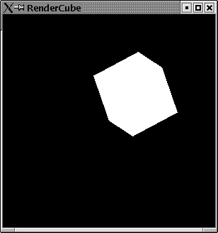
6.5.1 Defining a light source
For rendering three dimensional objects it is not enough to specifiy
their shapes and your viewing position. Crucial is the way the objects
are illuminated. In order to get a three dimensional viesual effect on
your two dimensional computer screen, it needs to be defined what kind
of light source lights the object.
A light source can be specified fairly easy. First you need to set the
state variable lighting to the value Enabled. Then
you need to specify the position of your light source. This can
be done by setting a special position state variable,
e.g. by
position (Light 0) $= Vertex4 0.8 0 3.0 5.0.
And finally you need to turn the light source on by setting its state variable to enabled: light (Light 0) $= Enabled.
You might wonder, why the vertex for the light source position has
four parameters. The forth parameter is a value by which the other
three (the x, y, z coordinates) get divided.
position (Light 0) $= Vertex4 0.8 0 3.0 5.0.
And finally you need to turn the light source on by setting its state variable to enabled: light (Light 0) $= Enabled.
Example:
Now we can render a cube with a defined light source:
LightCube
import Graphics.Rendering.OpenGL
import Graphics.UI.GLUT  as GLUT

import Cube

main = do
  (progName,_) <-  getArgsAndInitialize

  depthFunc $= Just Less

  createWindow progName

  lighting $= Enabled
  position (Light 0) $= Vertex4 1 0.4 0.8  1
  light (Light 0) $= Enabled

  displayCallback $= display
  mainLoop

display = do
  clear [ColorBuffer]
  rotate 40 (Vector3 1 1 (1::GLfloat))
  cube 0.5
  loadIdentity
  flush
The resulting window can be found in figure 6.10. Now we can identify a bit more the cube.
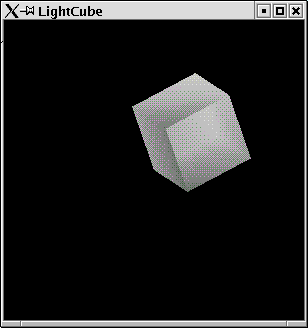
6.5.2 Tux the Penguin
Let us render some cute object: Tux the penguin. We will roughly use the data
from the OpenGL
game tuxracer.
The nice thing about a penguin is, that you can built it almost completely out
of spheres. We will render Tux simply by rendering spheres, which are scaled
to different forms and moved to the correct position.
Overall Setup
Tux
import Graphics.Rendering.OpenGL as OpenGL
import Graphics.UI.GLUT  as GLUT

import OrbitPointOfView
import StateUtil

main = do
  (progName,_) <-  getArgsAndInitialize
  initialDisplayMode $= [WithDepthBuffer,DoubleBuffered]
  pPos <- new (90::Int,270::Int,1.0)
  depthFunc $= Just Less
  createWindow progName

  lighting  $= Enabled
  normalize $= Enabled
  depthFunc $= Just Less

  position (Light 0) $= Vertex4 0 0 (10) 0
  ambient (Light 0) $= Color4 1 1 1 1
  diffuse (Light 0) $= Color4 1 1 1 1
  specular (Light 0) $= Color4 1 1 1 1
  light (Light 0) $= Enabled

  displayCallback $= display pPos
  keyboardMouseCallback $= Just (keyboard pPos)
  reshapeCallback $= Just reshape
  mainLoop

keyboard pPos c _  _ _ = keyForPos pPos c
The main display function clears the necessary buffers and calls the main
function for rendering the penguin Tux.
Tux
display pPos = do
  loadIdentity
  clearColor $= Color4 1 0 0 1
  setPointOfView pPos
  clear [ColorBuffer,DepthBuffer]
  tux
  swapBuffers
Auxilliary Functions
We will use some auxilliary functions. First of all a function, which renders a
scaled sphere.
Tux
sphere r xs ys zs = do
  scal xs ys zs
  createSphere r

createSphere r = renderObject Solid $Sphere' r 50 50

scal:: GLfloat -> GLfloat -> GLfloat -> IO ()
scal x y z = scale x y z
Furthermore some functions for easy translate and rotate transformations:
Tux
transl:: GLfloat -> GLfloat -> GLfloat -> IO ()
transl x y z= translate$Vector3 x y z

rota:: GLfloat -> GLfloat -> GLfloat -> GLfloat -> IO ()
rota a x y z  = rotate a $ Vector3 x y z

rotateZ a = rota a 0 0 1
rotateY a = rota a 0 1 0
rotateX a = rota a 1 0 0
And eventually some functions to set the material properties for the different
parts of a penguin.
Tux
crMat (rd,gd,bd) (rs,gs,bs) exp = do
  materialDiffuse   Front $= Color4 rd gd bd  1.0
  materialAmbient   Front $= Color4 rd gd bd  1.0
  materialSpecular  Front $= Color4 rs gs bs  1.0
  materialShininess Front $= exp

  materialDiffuse   Back $= Color4 rd gd bd  1.0
  materialSpecular  Back $= Color4 rs gs bs  1.0
  materialShininess Back $= exp

whitePenguin = crMat (0.58, 0.58, 0.58)(0.2, 0.2, 0.2) 50.0
blackPenguin = crMat (0.1, 0.1, 0.1)   (0.5, 0.5, 0.5) 20.0
beakColour   = crMat (0.64, 0.54, 0.06)(0.4, 0.4, 0.4) 5
nostrilColour= crMat (0.48039, 0.318627, 0.033725)(0.0,0.0,0.0) 1
irisColour   = crMat (0.01, 0.01, 0.01)(0.4, 0.4, 0.4) 90.0
Torso and Head
The neck and torso of a penguin are almost black spheres with some white front
parts. We will modell such figures by setting s white sphere in front of a
black sphere.
Tux
makeBody = do
  preservingMatrix$do
    blackPenguin
    sphere 1 0.95 1.0 0.8
  preservingMatrix$do
    whitePenguin
    transl 0 0 0.17
    sphere 1 0.8 0.9 0.7
The resulting image can be found in figure 6.11.
Torso and shoulders are scaled body parts:
Tux
createTorso = preservingMatrix$do
  scal 0.9 0.9 0.9
  makeBody

createShoulders = preservingMatrix$do
  transl 0 0.4 0.05
  leftArm
  rightArm
  scal 0.72 0.72 0.72
  makeBody
The resulting image for torso and shoulders
can be found in figure 6.12.
Tux
createNeck = preservingMatrix$do
 transl 0 0.9 0.07
 createHead
 rotateY 90
 blackPenguin
 sphere 0.8 0.45 0.5 0.45
 transl 0 (-0.08) 0.35
 whitePenguin
 sphere 0.66 0.8 0.9 0.7

createHead = preservingMatrix$do
 transl 0 0.3 0.07
 createBeak
 createEyes
 rotateY 90
 blackPenguin
 sphere 1 0.42 0.5 0.42

createBeak = do
  preservingMatrix$do
    transl 0 (-0.205) 0.3
    rotateX 10
    beakColour
    sphere 0.8 0.23 0.12 0.4
  preservingMatrix$do
    beakColour
    transl 0 (-0.23) 0.3
    rotateX 10
    sphere 0.66 0.21 0.17 0.38
Eyes
Tux
createEyes = preservingMatrix$do
  leftEye
  leftIris
  rightEye
  rightIris

leftEye = preservingMatrix$do
  transl 0.13 (-0.03) 0.38
  rotateY 18
  rotateZ 5
  rotateX 5
  whitePenguin
  sphere 0.66 0.1 0.13 0.03

rightEye = preservingMatrix$do
  transl (-0.13) (-0.03) 0.38
  rotateY (-18)
  rotateZ (-5)
  rotateX 5
  whitePenguin
  sphere 0.66 0.1 0.13 0.03

leftIris = preservingMatrix$do
  transl 0.12 (-0.045) 0.4
  rotateY 18
  rotateZ 5
  rotateX 5
  irisColour
  sphere 0.66 0.055 0.07 0.03

rightIris = preservingMatrix$do
  transl (-0.12) (-0.045) 0.4
  rotateY (-18)
  rotateZ (-5)
  rotateX 5
  irisColour
  sphere 0.66 0.055 0.07 0.03
Legs
Tux
leftArm = preservingMatrix$do
  rotateY 180
  transl (-0.56) 0.3 0
  rotateZ 45
  rotateX 90
  leftForeArm
  blackPenguin
  sphere 0.66 0.34 0.1 0.2

rightArm = preservingMatrix$do
  transl (-0.56) 0.3 0
  rotateZ 45
  rotateX(-90)
  rightForeArm
  blackPenguin
  sphere 0.66 0.34 0.1 0.2

leftForeArm = preservingMatrix$do
  transl (-0.23) 0 0
  rotateZ 20
  rotateX 90
  leftHand
  blackPenguin
  sphere 0.66 0.3 0.07 0.15

rightForeArm = leftForeArm

leftHand = preservingMatrix$do
  transl (-0.24) 0 0
  rotateZ 20
  rotateX 90
  blackPenguin
  sphere 0.5 0.12 0.05 0.12

leftTigh = preservingMatrix$do
  rotateY 180
  transl (-0.28) (-0.8) 0
  rotateY 110
  leftHipBall
  leftCalf

  rotateY (-110)
  transl 0 (-0.1) 0
  beakColour
  sphere 0.5 0.07 0.3 0.07

leftHipBall = preservingMatrix$do
  blackPenguin
  sphere 0.5 0.09 0.18 0.09

rightTigh = preservingMatrix$do
  transl (-0.28) (-0.8) 0
  rotateY (-110)
  rightHipBall
  rightCalf

  transl 0 (-0.1) 0
  beakColour
  sphere 0.5 0.07 0.3 0.07

rightHipBall = preservingMatrix$do
  blackPenguin
  sphere 0.5 0.09 0.18 0.09

leftCalf = preservingMatrix$do
 transl 0 (-0.21) 0
 rotateY 90
 leftFoot
 beakColour
 sphere 0.5 0.06 0.18 0.06

rightCalf = preservingMatrix$do
 transl 0 (-0.21) 0
 rightFoot
 beakColour
 sphere 0.5 0.06 0.18 0.06
Feet
Tux
foot = preservingMatrix$do
  scal  1.1 1.0 1.3
  beakColour
  footBase
  toe1
  toe2
  toe3

footBase = preservingMatrix$do
  sphere 0.66 0.25 0.08 0.18

toe1 = preservingMatrix$do
  transl (-0.07) 0 0.1
  rotateY 30
  scal 0.27 0.07 0.11
  createSphere 0.66

toe2 = preservingMatrix$do
 transl (-0.07) 0 (-0.1)
 rotateY (-30)
 sphere 0.66  0.27 0.07 0.11

toe3 = preservingMatrix$do
  transl (-0.08) 0 0
  sphere 0.66  0.27 0.07 0.10

leftFoot = preservingMatrix$do
  transl 0 (-0.09) 0
  rotateY (100)
  foot

rightFoot = preservingMatrix$do
  transl 0 (-0.09) 0
  rotateY 180
  foot
The resulting image can be found in figure 6.13.
Tail
Tux
createTail = preservingMatrix$ do
  transl 0 (-0.4) (-0.5)
  rotateX (-60)
  transl 0 0.15 0
  blackPenguin
  sphere 0.5 0.2 0.3 0.1
The complete penguin
We can use all the parts to define Tux.
Tux
tux = preservingMatrix$do
  scale 0.35 0.35 (0.35::GLfloat)
  rotateY (-180)
  rotateZ (-180)
  createTorso
  createShoulders
  createNeck
  leftTigh
  rightTigh
  createTail
The resulting window can be found in figure 6.14.
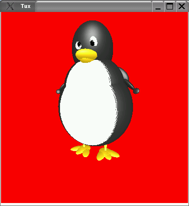
Index
Haskell ExamplesList of Figures
1.1 A simple polygon.2.1 Lines between points.
2.2 A loop of lines.
2.3 A strip in terms of lines.
2.4 Triangles.
2.5 A triangle strip.
2.6 A triangle strip.
2.7 Quads.
2.8 QuadStrips.
2.9 10 points on a circle.
2.10 Rendering a full circle.
2.11 A filled circle.
2.12 A simple ring shape.
2.13 Points of a large size.
2.14 Thick stippled lines.
2.15 A triangle with different vertex colors
2.16 RenderStar
2.17 A tea pot.
3.1 Rings translated to different positions.
3.2 Squares translated and rotated.
3.3 A coffee pot.
3.4 Different compositions of translation and rotation.
3.5 Applying shear to some shapes.
3.6 a Side of Rubik's Cube with further transformations applied to it.
4.1 Enlarging a window with the empty reshape function.
4.2 A Viewport smaller than the window.
4.3 Two windows with different projection.
5.1 Pong in action.
6.1 Third dimension not correctly taken into account.
6.2 Third dimension correctly taken into account by use of depth function.
6.3 Two squares in orthographic projection.
6.4 Perspective projection with frustum.
6.5 Two squares in perspective projection.
6.6 Perspective projection.
6.7 A view of the colored cube,
6.8 Rubik's Cube in action.
6.9 An unlit cube.
6.10 A lit cube.
6.11 Basic part for a penguin torso.
6.12 Penguin torso and shoulders.
6.13 A penguin foot.
6.14 Tux the penguin..
Bibliography
- []
- Norman Chin, Chris Frazier, Paul Ho, Zicheng Lui, and Kevin P. Smith. The OpenGL Graphics System Utility Library, 1998. ftp://ftp.sgi.com/opengl/doc/opengl1.2/glu1.3.ps.
- []
- Mark J. Kilgard. The OpenGL Utility Toolkit (GLUT), 1996. www.opengl.org/developers/documentation/glut/glut-3.spec.ps.
- []
- Simon L. Peyton Jones and Philip Wadler. Imperative functional programming. In Proceedings 20th Symposium on Principles of Programming Languages, pages 71-84, Charleston, South Carolina, 1993. ACM.
- []
- P. Wadler. Comprehending monads. In Proceedings of Symposium on Lisp and Functional Programming, pages 61-78, Nice, France, June 1990. ACM.
- []
- Mason Woo, OpenGL Architecture Review Board, Jackie Neider, Tom Davis, and Dave Shreiner. OpenGL Programming Guide 3rd Edition. Addison-Wesley, Reading, MA, 1997.